Kaggle 경진대회: Child Mind Institute — Problematic Internet Use
※ 개요
본 글은 Kaggle 경진대회: Child Mind Institute — Problematic Internet Use 의 수상코드를 분석 및 학습하는 것입니다.
'''
캐글 경진대회 : Child Mind Institute — Problematic Internet Use
데이터 세트 : Healthy Brain Network(HBN) 데이터 세트는 임상 및 연구 검진을 모두 거친 약 5,000명의 5~22세의 임상 샘플, parquet가속도계(액티그래피) 시리즈를 포함하는 파일과 train 및 test 파일
목적 : 심각도 장애 지수(Severity Impairment Index , sii)를 예측
주의사항은 PCIAT-PCIAT_Total 피처(데이터셋 내의 Parent-Child Internet Addiction Test- 강박성, 현실도피주의, 의존성을 포함하여 인터넷 강박적 사용과 관련된 특성과 행동을 측정하는 20문항 척도를 합산한 점수)에서 파생된 값이 sii임
'''
※ 머신러닝 예측 파이프 라인
[Start]
   │
   ▼
[Load Raw Data (train, test, series)]
   │
   ▼
[Clean Features]
   - Clip 이상치
   - NaN 처리
   │
   ▼
[Feature Engineering]
   - Age group assign
   - BMI 정규화
   - FGC zone 평균, 최대/최소
   - Push-up, Curl-up 정규화 등
   │
   ▼
[Time-Series Feature Extraction]
   - 'series_*.parquet' 파일 병렬 처리
   - 낮/밤/전체 마스크 통계값 추출
   │
   ▼
[StandardScaler]
   - train 기준 평균-표준편차 정규화
   │
   ▼
[PCA (차원 축소)]
   - n_components=15
   - id 기준 merge
   │
   ▼
[Missing Value Imputation]
   - LassoCV 기반 모델로 결측값 예측
   - 결측률 높을 경우 평균 대체
   │
   ▼
[Discretization (Binning)]
   - 연속형 변수 10개 구간으로 분할
   - train + test 기준 quantile cut
   │
   ▼
[Feature Selection]
   - test에 없는 PCIAT 변수들 제외
   │
   ▼
[Train/Validation Split (Stratified K-Fold)]
   - 'sii' 기준 층화 샘플링
   │
   ▼
[Model Training (CV)]
   - LGBM / XGBoost / CatBoost / ExtraTrees
   - sample_weight 적용
   │
   ▼
[Threshold Optimization]
   - OOF 예측 → 최적 임계값으로 분류 변환
   - QWK 최적화 (Powell 방식)
   │
   ▼
[Ensembling]
   ├── [Voting Ensemble]
   └── [Weighted Average Ensemble]
   │
   ▼
[Evaluate OOF]
   - Confusion Matrix, QWK 점수 확인
   │
   ▼
[Final Prediction on Test Set]
   - 최적 threshold 적용 후 예측
   │
   ▼
[Save Submission File (submission.csv)]
1. set up
import numpy as np
import pandas as pd
import os
from sklearn.base import clone
from sklearn.metrics import cohen_kappa_score, make_scorer, confusion_matrix
from sklearn.model_selection import StratifiedKFold, KFold, train_test_split
from sklearn.preprocessing import StandardScaler
from sklearn.decomposition import PCA
from scipy.optimize import minimize
from scipy import stats
from concurrent.futures import ThreadPoolExecutor
from tqdm import tqdm
import warnings
from sklearn.linear_model import ElasticNetCV, LassoCV, Lasso, LinearRegression
from sklearn.ensemble import ExtraTreesRegressor, RandomForestRegressor
from lightgbm import LGBMRegressor
from xgboost import XGBRegressor
from catboost import CatBoostRegressor
import optuna
import matplotlib.pyplot as plt
import seaborn as sns
import numpy as np
import random
import pickle

warnings.filterwarnings('ignore')
SEED = 9365
n_splits = 10
optimize_params = False
n_trials = 25 # n_trials for optuna
voting = True
base_thresholds = [30, 50, 80]# Load datasets
train = pd.read_csv('/content/drive/MyDrive/child-mind-institute-problematic-internet-use/train.csv')
test = pd.read_csv('/content/drive/MyDrive/child-mind-institute-problematic-internet-use/test.csv')
train.info()<class 'pandas.core.frame.DataFrame'>
RangeIndex: 3960 entries, 0 to 3959
Data columns (total 82 columns):
# Column Non-Null Count Dtype
--- ------ -------------- -----
0 id 3960 non-null object
1 Basic_Demos-Enroll_Season 3960 non-null object
2 Basic_Demos-Age 3960 non-null int64
3 Basic_Demos-Sex 3960 non-null int64
4 CGAS-Season 2555 non-null object
5 CGAS-CGAS_Score 2421 non-null float64
6 Physical-Season 3310 non-null object
7 Physical-BMI 3022 non-null float64
8 Physical-Height 3027 non-null float64
9 Physical-Weight 3076 non-null float64
10 Physical-Waist_Circumference 898 non-null float64
11 Physical-Diastolic_BP 2954 non-null float64
12 Physical-HeartRate 2967 non-null float64
13 Physical-Systolic_BP 2954 non-null float64
14 Fitness_Endurance-Season 1308 non-null object
15 Fitness_Endurance-Max_Stage 743 non-null float64
16 Fitness_Endurance-Time_Mins 740 non-null float64
17 Fitness_Endurance-Time_Sec 740 non-null float64
18 FGC-Season 3346 non-null object
19 FGC-FGC_CU 2322 non-null float64
20 FGC-FGC_CU_Zone 2282 non-null float64
21 FGC-FGC_GSND 1074 non-null float64
22 FGC-FGC_GSND_Zone 1062 non-null float64
23 FGC-FGC_GSD 1074 non-null float64
24 FGC-FGC_GSD_Zone 1063 non-null float64
25 FGC-FGC_PU 2310 non-null float64
26 FGC-FGC_PU_Zone 2271 non-null float64
27 FGC-FGC_SRL 2305 non-null float64
28 FGC-FGC_SRL_Zone 2267 non-null float64
29 FGC-FGC_SRR 2307 non-null float64
30 FGC-FGC_SRR_Zone 2269 non-null float64
31 FGC-FGC_TL 2324 non-null float64
32 FGC-FGC_TL_Zone 2285 non-null float64
33 BIA-Season 2145 non-null object
34 BIA-BIA_Activity_Level_num 1991 non-null float64
35 BIA-BIA_BMC 1991 non-null float64
36 BIA-BIA_BMI 1991 non-null float64
37 BIA-BIA_BMR 1991 non-null float64
38 BIA-BIA_DEE 1991 non-null float64
39 BIA-BIA_ECW 1991 non-null float64
40 BIA-BIA_FFM 1991 non-null float64
41 BIA-BIA_FFMI 1991 non-null float64
42 BIA-BIA_FMI 1991 non-null float64
43 BIA-BIA_Fat 1991 non-null float64
44 BIA-BIA_Frame_num 1991 non-null float64
45 BIA-BIA_ICW 1991 non-null float64
46 BIA-BIA_LDM 1991 non-null float64
47 BIA-BIA_LST 1991 non-null float64
48 BIA-BIA_SMM 1991 non-null float64
49 BIA-BIA_TBW 1991 non-null float64
50 PAQ_A-Season 475 non-null object
51 PAQ_A-PAQ_A_Total 475 non-null float64
52 PAQ_C-Season 1721 non-null object
53 PAQ_C-PAQ_C_Total 1721 non-null float64
54 PCIAT-Season 2736 non-null object
55 PCIAT-PCIAT_01 2733 non-null float64
56 PCIAT-PCIAT_02 2734 non-null float64
57 PCIAT-PCIAT_03 2731 non-null float64
58 PCIAT-PCIAT_04 2731 non-null float64
59 PCIAT-PCIAT_05 2729 non-null float64
60 PCIAT-PCIAT_06 2732 non-null float64
61 PCIAT-PCIAT_07 2729 non-null float64
62 PCIAT-PCIAT_08 2730 non-null float64
63 PCIAT-PCIAT_09 2730 non-null float64
64 PCIAT-PCIAT_10 2733 non-null float64
65 PCIAT-PCIAT_11 2734 non-null float64
66 PCIAT-PCIAT_12 2731 non-null float64
67 PCIAT-PCIAT_13 2729 non-null float64
68 PCIAT-PCIAT_14 2732 non-null float64
69 PCIAT-PCIAT_15 2730 non-null float64
70 PCIAT-PCIAT_16 2728 non-null float64
71 PCIAT-PCIAT_17 2725 non-null float64
72 PCIAT-PCIAT_18 2728 non-null float64
73 PCIAT-PCIAT_19 2730 non-null float64
74 PCIAT-PCIAT_20 2733 non-null float64
75 PCIAT-PCIAT_Total 2736 non-null float64
76 SDS-Season 2618 non-null object
77 SDS-SDS_Total_Raw 2609 non-null float64
78 SDS-SDS_Total_T 2606 non-null float64
79 PreInt_EduHx-Season 3540 non-null object
80 PreInt_EduHx-computerinternet_hoursday 3301 non-null float64
81 sii 2736 non-null float64
dtypes: float64(68), int64(2), object(12)
memory usage: 2.5+ MB
series_train.parquer 파일 1개 예시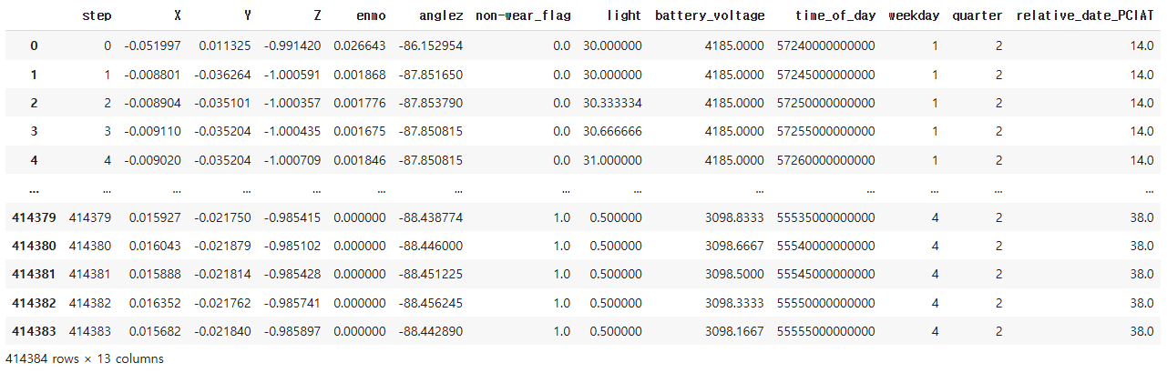
2. Preprocessing
1) PCA 차원 축소
def perform_pca(train, test, n_components=None, random_state=42):

    pca = PCA(n_components=n_components, random_state=random_state)
    train_pca = pca.fit_transform(train)
    test_pca = pca.transform(test)

    explained_variance_ratio = pca.explained_variance_ratio_
    print(f"Explained variance ratio of the components:\n {explained_variance_ratio}")
    print(np.sum(explained_variance_ratio))

    train_pca_df = pd.DataFrame(train_pca, columns=[f'PC_{i+1}' for i in range(train_pca.shape[1])])
    test_pca_df = pd.DataFrame(test_pca, columns=[f'PC_{i+1}' for i in range(test_pca.shape[1])])

    return train_pca_df, test_pca_df, pca
※ 코드 분석
PCA로 피처수 축소하는 함수
[ Train/Test Data ]
        │
        ▼
[ perform_pca() ]
        │
        ├─ fit_transform(train) → train_pca_df (PC_1 ~ PC_n)
        ├─ transform(test) → test_pca_df
        └─ print(설명력)
2) 시계열 파일 피처에서 유의미한 통계값 추출
def time_features(df):
    # Convert time_of_day to hours
    df["hours"] = df["time_of_day"] // (3_600 * 1_000_000_000)
    # Basic features
    features = [
        df["non-wear_flag"].mean(),
        df["enmo"][df["enmo"] >= 0.05].sum(),
    ]

    # Define conditions for night, day, and no mask (full data)
    night = ((df["hours"] >= 22) | (df["hours"] <= 5))
    day = ((df["hours"] <= 20) & (df["hours"] >= 7))
    no_mask = np.ones(len(df), dtype=bool)

    # List of columns of interest and masks
    keys = ["enmo", "anglez", "light", "battery_voltage"]
    masks = [no_mask, night, day]

    # Helper function for feature extraction
    def extract_stats(data):
        return [
            data.mean(),
            data.std(),
            data.max(),
            data.min(),
            data.diff().mean(),
            data.diff().std()
        ]

    # Iterate over keys and masks to generate the statistics
    for key in keys:
        for mask in masks:
            filtered_data = df.loc[mask, key]
            features.extend(extract_stats(filtered_data))

    return features

# Code for parallelized computation of time series data from: Sheikh Muhammad Abdullah
# https://www.kaggle.com/code/abdmental01/cmi-best-single-model
def process_file(filename, dirname):
    # Process file and extract time features
    df = pd.read_parquet(os.path.join(dirname, filename, 'part-0.parquet'))
    df.drop('step', axis=1, inplace=True)
    return time_features(df), filename.split('=')[1]

def load_time_series(dirname) -> pd.DataFrame:
    # Load time series from directory in parallel
    ids = os.listdir(dirname)

    with ThreadPoolExecutor() as executor:
        results = list(tqdm(executor.map(lambda fname: process_file(fname, dirname), ids), total=len(ids)))

    stats, indexes = zip(*results)

    df = pd.DataFrame(stats, columns=[f"stat_{i}" for i in range(len(stats[0]))])
    df['id'] = indexes

    return df
※ 코드 분석
시간 시계열 데이터를 처리하고 통계 피처를 자동으로 추출하는 함수
START
  │
  ▼
[시계열 디렉토리 경로 지정: dirname]
  │
  ▼
[디렉토리 내 파일 목록 읽기]
  │
  ▼
[ThreadPoolExecutor 시작 → 각 파일에 대해 process_file() 실행]
  │
  ▼
┌────────────────────────────────────────────────────────────┐
│ process_file(filename, dirname)                            │
│ ┌────────────────────────────────────────────────────────┐ │
│ │ 파일 경로: os.path.join(dirname, filename, "part-0.parquet") │
│ │ 파일 읽기 → DataFrame(df)                              │
│ │ 컬럼 'step' 제거                                        │
│ │ 호출: time_features(df)                                │
│ └────────────────────────────────────────────────────────┘ │
│ 반환값: (특징 벡터 리스트, id 값)                           │
└────────────────────────────────────────────────────────────┘
  │
  ▼
┌────────────────────────────────────────────────────────────┐
│ time_features(df)                                          │
│ ┌────────────────────────────────────────────────────────┐ │
│ │ [1] 시간 정보 전처리:                                    │
│ │     df["hours"] = df["time_of_day"] // (3.6e12)         │
│ │                                                        │
│ │ [2] 기본 특징 생성                                      │
│ │     - non-wear 비율                                     │
│ │     - 움직임(enmo ≥ 0.05)의 합                          │
│ │                                                        │
│ │ [3] 시간대 마스크 설정:                                 │
│ │     - night: 22시~5시                                   │
│ │     - day: 7시~20시                                     │
│ │     - no_mask: 전체                                     │
│ │                                                        │
│ │ [4] 센서값별 통계 계산:                                 │
│ │     keys = [enmo, anglez, light, battery_voltage]       │
│ │     masks = [전체, night, day]                          │
│ │     → 각 조합별로 [mean, std, max, min, diff.mean, diff.std] │
│ └────────────────────────────────────────────────────────┘ │
│ 반환값: 총 26개의 통계 피처                                │
└────────────────────────────────────────────────────────────┘
  │
  ▼
[결과 (피처, id) 튜플 리스트로 모음]
  │
  ▼
[zip → 통계값 리스트(stat_x), id 리스트 구성]
  │
  ▼
[pd.DataFrame으로 변환 → "stat_0" ~ "stat_25" + id]
  │
  ▼
RETURN 완료된 Feature DataFrame
3) 피처 엔지니어링
def feature_engineering(df):
    season_cols = [col for col in df.columns if 'Season' in col]
    df = df.drop(season_cols, axis=1)

    # From here on own features
    def assign_group(age):
        thresholds = [5, 6, 7, 8, 10, 12, 14, 17, 22]
        for i, j in enumerate(thresholds):
            if age <= j:
                return i
        return np.nan

    # Age groups
    df["group"] = df['Basic_Demos-Age'].apply(assign_group)

    # BMI
    BMI_map = {0: 16.3,1: 15.9,2: 16.1,3: 16.8,4: 17.3,5: 19.2,6: 20.2,7: 22.3, 8: 23.6}
    df['BMI_mean_norm'] = df[['Physical-BMI', 'BIA-BIA_BMI']].mean(axis=1) / df["group"].map(BMI_map)

    # FGC zone aggregate
    zones = ['FGC-FGC_CU_Zone', 'FGC-FGC_GSND_Zone', 'FGC-FGC_GSD_Zone',
             'FGC-FGC_PU_Zone', 'FGC-FGC_SRL_Zone', 'FGC-FGC_SRR_Zone',
             'FGC-FGC_TL_Zone']

    df['FGC_Zones_mean'] = df[zones].mean(axis=1)
    df['FGC_Zones_min'] = df[zones].min(axis=1)
    df['FGC_Zones_max'] = df[zones].max(axis=1)

    # Grip
    GSD_max_map = {0: 9, 1: 9, 2: 9, 3: 9, 4: 16.2, 5: 19.9, 6: 26.1, 7: 31.3, 8: 35.4}
    GSD_min_map = {0: 9, 1: 9, 2: 9, 3: 9, 4: 14.4, 5: 17.8, 6: 23.4, 7: 27.8, 8: 31.1}

    df['GS_max'] = df[['FGC-FGC_GSND', 'FGC-FGC_GSD']].max(axis=1) / df["group"].map(GSD_max_map)
    df['GS_min'] = df[['FGC-FGC_GSND', 'FGC-FGC_GSD']].min(axis=1) / df["group"].map(GSD_min_map)

    # Curl-ups, push-ups, trunk-lifts... normalized based on age-group
    cu_map = {0: 1.0, 1: 3.0, 2: 5.0, 3: 7.0, 4: 10.0, 5: 14.0, 6: 20.0, 7: 20.0, 8: 20.0}
    pu_map = {0: 1.0, 1: 2.0, 2: 3.0, 3: 4.0, 4: 5.0, 5: 7.0, 6: 8.0, 7: 10.0, 8: 14.0}
    tl_map = {0: 8.0, 1: 8.0, 2: 8.0, 3: 9.0, 4: 9.0, 5: 10.0, 6: 10.0, 7: 10.0, 8: 10.0}

    df["CU_norm"] = df['FGC-FGC_CU'] / df['group'].map(cu_map)
    df["PU_norm"] = df['FGC-FGC_PU'] / df['group'].map(pu_map)
    df["TL_norm"] = df['FGC-FGC_TL'] / df['group'].map(tl_map)

    # Reach
    df["SR_min"] = df[['FGC-FGC_SRL', 'FGC-FGC_SRR']].min(axis=1)
    df["SR_max"] = df[['FGC-FGC_SRL', 'FGC-FGC_SRR']].max(axis=1)

    # BIA Features
    # Energy Expenditure
    bmr_map = {0: 934.0, 1: 941.0, 2: 999.0, 3: 1048.0, 4: 1283.0, 5: 1255.0, 6: 1481.0, 7: 1519.0, 8: 1650.0}
    dee_map = {0: 1471.0, 1: 1508.0, 2: 1640.0, 3: 1735.0, 4: 2132.0, 5: 2121.0, 6: 2528.0, 7: 2566.0, 8: 2793.0}
    df["BMR_norm"] = df["BIA-BIA_BMR"] / df["group"].map(bmr_map)
    df["DEE_norm"] = df["BIA-BIA_DEE"] / df["group"].map(dee_map)
    df["DEE_BMR"] = df["BIA-BIA_DEE"] - df["BIA-BIA_BMR"]

    # FMM
    ffm_map = {0: 42.0, 1: 43.0, 2: 49.0, 3: 54.0, 4: 60.0, 5: 76.0, 6: 94.0, 7: 104.0, 8: 111.0}
    df["FFM_norm"] = df["BIA-BIA_FFM"] / df["group"].map(ffm_map)

    # ECW ICW
    df["ICW_ECW"] = df["BIA-BIA_ECW"] / df["BIA-BIA_ICW"]

    drop_feats = ['FGC-FGC_GSND', 'FGC-FGC_GSD', 'FGC-FGC_CU_Zone', 'FGC-FGC_GSND_Zone', 'FGC-FGC_GSD_Zone',
                  'FGC-FGC_PU_Zone', 'FGC-FGC_SRL_Zone', 'FGC-FGC_SRR_Zone', 'FGC-FGC_TL_Zone',
                  'Physical-BMI', 'BIA-BIA_BMI', 'FGC-FGC_CU', 'FGC-FGC_PU', 'FGC-FGC_TL', 'FGC-FGC_SRL', 'FGC-FGC_SRR',
                 'BIA-BIA_BMR', 'BIA-BIA_DEE', 'BIA-BIA_Frame_num', "BIA-BIA_FFM"]
    df = df.drop(drop_feats, axis=1)
    return df
※ 코드 분석
기존의 데이터에서 신규 파생변수를 만들어내고 불필요한 컬럼을 제거하는 과정
[1] 시작: 원본 데이터프레임 (df)
 └─ 포함된 컬럼 예: 'Basic_Demos-Age', 'Physical-BMI', 'FGC-FGC_CU_Zone', 'BIA-BIA_BMR', ...

│
▼

[2] 시즌 컬럼 제거
 └─ 동작: 'Season'이라는 단어가 포함된 컬럼들 제거
 └─ 예: 'FGC-Season', 'PAQ_A-Season' 등 제거됨

│
▼

[3] 나이 기반 그룹핑 (group 컬럼 생성)
 └─ 입력: 'Basic_Demos-Age'
 └─ 연령대 기준: [5, 6, 7, 8, 10, 12, 14, 17, 22]
 └─ 출력: group = 0 ~ 8의 정수

│
▼

[4] BMI 정규화 피처 생성 (BMI_mean_norm)
 └─ 입력: ['Physical-BMI', 'BIA-BIA_BMI']
 └─ 처리: 평균 → group에 따른 기준값으로 나눔
 └─ 출력: BMI_mean_norm

│
▼

[5] FGC Zone 통계 3개 생성
 └─ 입력: 7개의 ZONE 컬럼
     ['FGC-FGC_CU_Zone', ..., 'FGC-FGC_TL_Zone']
 └─ 출력:
     - FGC_Zones_mean
     - FGC_Zones_min
     - FGC_Zones_max

│
▼

[6] 악력 관련 정규화 피처 생성 (GS_min, GS_max)
 └─ 입력: 'FGC-FGC_GSND', 'FGC-FGC_GSD'
 └─ 처리: group 기준으로 정규화
 └─ 출력: GS_min, GS_max

│
▼

[7] 근력/근지구력 정규화
 └─ 입력: ['FGC-FGC_CU', 'FGC-FGC_PU', 'FGC-FGC_TL']
 └─ 처리: 각각 cu_map, pu_map, tl_map 사용하여 group 기준 정규화
 └─ 출력: CU_norm, PU_norm, TL_norm

│
▼

[8] 유연성 검사 정리
 └─ 입력: 'FGC-FGC_SRL', 'FGC-FGC_SRR'
 └─ 출력: SR_min, SR_max

│
▼

[9] 에너지 관련 피처 생성
 └─ 입력: 'BIA-BIA_BMR', 'BIA-BIA_DEE'
 └─ 처리:
     - BMR_norm = BMR / 기준값
     - DEE_norm = DEE / 기준값
     - DEE_BMR = DEE - BMR

│
▼

[10] 체성분 정규화 피처
 └─ 입력: 'BIA-BIA_FFM' (제지방량)
 └─ 처리: group 기준 정규화 → FFM_norm

│
▼

[11] 수분 비율 계산
 └─ 입력: 'BIA-BIA_ECW', 'BIA-BIA_ICW'
 └─ 출력: ICW_ECW = ECW / ICW

│
▼

[12] 파생변수 생성에 사용한 원본 컬럼 제거
 └─ 제거 예시:
     - 'FGC-FGC_CU', 'BIA-BIA_BMR', 'Physical-BMI', 'FGC-FGC_GSND' 등등

│
▼

[13] 최종 출력: 가공된 데이터프레임 반환
 └─ 파생 변수 + 정제된 원본 컬럼만 포함
 └─ 모델 학습에 적합한 형태로 변형 완료
4) 시계열 데이터 기반 통계 피처를 생성하고, 차원 축소 후 train/test 데이터에 병합하는 전처리 코드
train_ts = load_time_series("/content/drive/MyDrive/child-mind-institute-problematic-internet-use/series_train.parquet")
test_ts = load_time_series("/content/drive/MyDrive/child-mind-institute-problematic-internet-use/series_test.parquet")

df_train = train_ts.drop('id', axis=1)
df_test = test_ts.drop('id', axis=1)

scaler = StandardScaler()
df_train = pd.DataFrame(scaler.fit_transform(df_train), columns=df_train.columns)
df_test = pd.DataFrame(scaler.transform(df_test), columns=df_test.columns)

for c in df_train.columns:
    m = np.mean(df_train[c])
    df_train[c].fillna(m, inplace=True)
    df_test[c].fillna(m, inplace=True)

print(df_train.shape)

df_train_pca, df_test_pca, pca = perform_pca(df_train, df_test, n_components=15, random_state=SEED)

df_train_pca['id'] = train_ts['id']
df_test_pca['id'] = test_ts['id']

train = pd.merge(train, df_train_pca, how="left", on='id')
test = pd.merge(test, df_test_pca, how="left", on='id')
train.shape
100%|██████████| 996/996 [04:20<00:00, 3.82it/s]
100%|██████████| 2/2 [00:01<00:00, 1.80it/s](996, 74)
Explained variance ratio of the components:
[0.22219101 0.11409028 0.0661572 0.06115724 0.05273775 0.04588977
0.04282018 0.03804032 0.03464056 0.0299413 0.02582865 0.02512208
0.02316028 0.02173871 0.01984202]
0.8233573434410545
(3960, 97)
※ 코드 분석
지금까지 만들었던 함수들로 시계열 파일 전처리 시행 후 train, test 파일에 병합
📁 시계열 파일 (series_train.parquet, series_test.parquet)
        ↓
📈 load_time_series → 통계 피처 생성 (stat_0 ~ stat_n)
        ↓
📏 정규화 (StandardScaler)
        ↓
❓ 결측값 평균 대체
        ↓
🔄 PCA (PC_1 ~ PC_15 생성)
        ↓
🔗 train / test 에 병합 (id 기준 left join)
5) 이상치 처리, 피처엔지니어링 실행
def clean_features(df):
    # Remove highly implausible values

    # Clip Grip
    df[['FGC-FGC_GSND', 'FGC-FGC_GSD']] = df[['FGC-FGC_GSND', 'FGC-FGC_GSD']].clip(lower=9, upper=60)
    # Remove implausible body-fat
    df["BIA-BIA_Fat"] = np.where(df["BIA-BIA_Fat"] < 5, np.nan, df["BIA-BIA_Fat"])
    df["BIA-BIA_Fat"] = np.where(df["BIA-BIA_Fat"] > 60, np.nan, df["BIA-BIA_Fat"])
    # Basal Metabolic Rate
    df["BIA-BIA_BMR"] = np.where(df["BIA-BIA_BMR"] > 4000, np.nan, df["BIA-BIA_BMR"])
    # Daily Energy Expenditure
    df["BIA-BIA_DEE"] = np.where(df["BIA-BIA_DEE"] > 8000, np.nan, df["BIA-BIA_DEE"])
    # Bone Mineral Content
    df["BIA-BIA_BMC"] = np.where(df["BIA-BIA_BMC"] <= 0, np.nan, df["BIA-BIA_BMC"])
    df["BIA-BIA_BMC"] = np.where(df["BIA-BIA_BMC"] > 10, np.nan, df["BIA-BIA_BMC"])
    # Fat Free Mass Index
    df["BIA-BIA_FFM"] = np.where(df["BIA-BIA_FFM"] <= 0, np.nan, df["BIA-BIA_FFM"])
    df["BIA-BIA_FFM"] = np.where(df["BIA-BIA_FFM"] > 300, np.nan, df["BIA-BIA_FFM"])
    # Fat Mass Index
    df["BIA-BIA_FMI"] = np.where(df["BIA-BIA_FMI"] < 0, np.nan, df["BIA-BIA_FMI"])
    # Extra Cellular Water
    df["BIA-BIA_ECW"] = np.where(df["BIA-BIA_ECW"] > 100, np.nan, df["BIA-BIA_ECW"])
    # Intra Cellular Water
    # df["BIA-BIA_ICW"] = np.where(df["BIA-BIA_ICW"] > 100, np.nan, df["BIA-BIA_ICW"])
    # Lean Dry Mass
    df["BIA-BIA_LDM"] = np.where(df["BIA-BIA_LDM"] > 100, np.nan, df["BIA-BIA_LDM"])
    # Lean Soft Tissue
    df["BIA-BIA_LST"] = np.where(df["BIA-BIA_LST"] > 300, np.nan, df["BIA-BIA_LST"])
    # Skeletal Muscle Mass
    df["BIA-BIA_SMM"] = np.where(df["BIA-BIA_SMM"] > 300, np.nan, df["BIA-BIA_SMM"])
    # Total Body Water
    df["BIA-BIA_TBW"] = np.where(df["BIA-BIA_TBW"] > 300, np.nan, df["BIA-BIA_TBW"])

    return df

train = clean_features(train)
test = clean_features(test)

train = feature_engineering(train)
test = feature_engineering(test)
※ 코드 분석
신체 수치가 비현실적일 경우 제거하는 코드
[입력: 원본 DataFrame df]
        │
        ▼
┌────────────────────────────────────────────┐
│            Grip Strength 정제             │
│ ['FGC-FGC_GSND', 'FGC-FGC_GSD'] 컬럼 →     │
│ 9kg 이하, 60kg 이상 값을 → 9~60으로 clip  │
└────────────────────────────────────────────┘
        │
        ▼
┌────────────────────────────────────────────┐
│        체지방률(BIA-BIA_Fat) 이상치 제거    │
│ 5% 미만 또는 60% 초과인 값 → NaN           │
└────────────────────────────────────────────┘
        │
        ▼
┌────────────────────────────────────────────┐
│        기초대사량(BIA-BIA_BMR) 정제        │
│ 4000 kcal 초과 값 → NaN                    │
└────────────────────────────────────────────┘
        │
        ▼
┌────────────────────────────────────────────┐
│       일일에너지소비량(BIA-BIA_DEE) 정제    │
│ 8000 kcal 초과 값 → NaN                    │
└────────────────────────────────────────────┘
        │
        ▼
┌────────────────────────────────────────────┐
│    골밀도(BIA-BIA_BMC) 정제                │
│ 0 이하 or 10 이상인 값 → NaN              │
└────────────────────────────────────────────┘
        │
        ▼
┌────────────────────────────────────────────┐
│  제지방질량지수(BIA-BIA_FFM) 정제         │
│ 0 이하 또는 300 초과 값 → NaN             │
└────────────────────────────────────────────┘
        │
        ▼
┌────────────────────────────────────────────┐
│     체지방지수(BIA-BIA_FMI) 정제           │
│ 0 미만 값 → NaN                            │
└────────────────────────────────────────────┘
        │
        ▼
┌────────────────────────────────────────────┐
│      체수분량(ECW, LDM, LST, SMM, TBW 등)  │
│ 각 항목별로 현실적으로 불가능한 값 제거  │
│ 예: SMM > 300kg → NaN                      │
└────────────────────────────────────────────┘
        │
        ▼
[출력: 이상치가 제거된 DataFrame 반환]
6) 연속형 변수들을 구간형(범주형) 데이터로 변환
def bin_data(train, test, columns, n_bins=10):
    # Combine train and test for consistent bin edges
    combined = pd.concat([train, test], axis=0)

    bin_edges = {}
    for col in columns:
        # Compute quantile bin edges
        edges = pd.qcut(combined[col], n_bins, retbins=True, labels=range(n_bins), duplicates="drop")[1]
        bin_edges[col] = edges

    # Apply the same bin edges to both train and test
    for col, edges in bin_edges.items():
        train[col] = pd.cut(
            train[col], bins=edges, labels=range(len(edges) - 1), include_lowest=True
        ).astype(float)
        test[col] = pd.cut(
            test[col], bins=edges, labels=range(len(edges) - 1), include_lowest=True
        ).astype(float)

    return train, test

# Usage example
columns_to_bin = [
    "PAQ_A-PAQ_A_Total", "BMR_norm", "DEE_norm", "GS_min", "GS_max", "BIA-BIA_FFMI",
    "BIA-BIA_BMC", "Physical-HeartRate", "BIA-BIA_ICW", "Fitness_Endurance-Time_Sec",
    "BIA-BIA_LDM", "BIA-BIA_SMM", "BIA-BIA_TBW", "DEE_BMR", "ICW_ECW"
]
train, test = bin_data(train, test, columns_to_bin, n_bins=10)
※ 코드 분석
[입력: train DataFrame, test DataFrame, binning할 컬럼 리스트]
        │
        ▼
┌───────────────────────────────────────────┐
│     train과 test 데이터를 세로로 합치기   │
│ → 전체 데이터에서 bin의 기준을 동일하게 설정 │
└───────────────────────────────────────────┘
        │
        ▼
┌───────────────────────────────────────────┐
│ 각 컬럼별로 분위수 기반으로 bin 경계 구하기 │
│ → pd.qcut()으로 quantile 기준 경계 추출      │
│ 예: 10분위 → 0~10%, 10~20%, ..., 90~100%     │
└───────────────────────────────────────────┘
        │
        ▼
┌────────────────────────────────────────────┐
│ 구한 bin 경계를 기준으로 각 값에 bin 번호 부여 │
│ → pd.cut() 사용 (각 데이터가 몇 분위인지)       │
│ 예: 7번째 분위수면 label 6                    │
└────────────────────────────────────────────┘
        │
        ▼
[출력: train, test에 구간형 숫자 값이 추가된 DataFrame 반환]
7) 사용할 피처(feature) 선택과 범주형 변수 처리
# Features to exclude, because they're not in test
exclude = ['PCIAT-Season', 'PCIAT-PCIAT_01', 'PCIAT-PCIAT_02', 'PCIAT-PCIAT_03',
           'PCIAT-PCIAT_04', 'PCIAT-PCIAT_05', 'PCIAT-PCIAT_06', 'PCIAT-PCIAT_07',
           'PCIAT-PCIAT_08', 'PCIAT-PCIAT_09', 'PCIAT-PCIAT_10', 'PCIAT-PCIAT_11',
           'PCIAT-PCIAT_12', 'PCIAT-PCIAT_13', 'PCIAT-PCIAT_14', 'PCIAT-PCIAT_15',
           'PCIAT-PCIAT_16', 'PCIAT-PCIAT_17', 'PCIAT-PCIAT_18', 'PCIAT-PCIAT_19',
           'PCIAT-PCIAT_20', 'PCIAT-PCIAT_Total', 'sii', 'id']

y_model = "PCIAT-PCIAT_Total" # Score, target for the model
y_comp = "sii" # Index, target of the competition
features = [f for f in train.columns if f not in exclude]

# Categorical features
# cat_c = ['Basic_Demos-Enroll_Season', 'CGAS-Season', 'Physical-Season', 'Fitness_Endurance-Season',
#           'FGC-Season', 'BIA-Season', 'PAQ_A-Season', 'PAQ_C-Season', 'SDS-Season', 'PreInt_EduHx-Season']
cat_c = []

for col in cat_c:
    a_map = {}
    all_unique = set(train[col].unique()) | set(test[col].unique())
    for i, value in enumerate(all_unique):
        a_map[value] = i

    train[col] = train[col].map(a_map)
    test[col] = test[col].map(a_map)

train = train[train["sii"].notna()] # Keep rows where target is available
※ 코드 분석
PCIAT 관련 피처들을 제외하는 이유는 해당 값으로 sii 값을 만들어내기 때문
(PCIAT 총 합계를 0~3 레이블로 분할 한 값 = sii)
즉, PCIAT값으로 학습을 하면 정답을 보고 학습을 하는것이기 때문에 데이터 누수에 해당
[train DataFrame] ─────────────┐
[test DataFrame] ──────┐       │
                       ▼       ▼
        ┌──────────────────────────────────────────┐
        │  ❌ 제외할 컬럼 리스트 정의 (test에 없는 컬럼 등) │
        └──────────────────────────────────────────┘
                       ▼
        ┌──────────────────────────────────────────┐
        │ 🎯 모델 타겟과 정답 레이블 컬럼 정의           │
        └──────────────────────────────────────────┘
                       ▼
        ┌──────────────────────────────────────────────┐
        │ ✅ 제외 컬럼을 빼고 모델에 넣을 features 선정     │
        └──────────────────────────────────────────────┘
                       ▼
        ┌──────────────────────────────────────────────┐
        │ 🧮 (선택적) 범주형 컬럼이 있으면 숫자로 매핑       │
        └──────────────────────────────────────────────┘
                       ▼
        ┌──────────────────────────────────────────────┐
        │ 🧹 'sii'가 결측치인 row 제거 (학습 타겟이 없는 데이터) │
        └──────────────────────────────────────────────┘
                       ▼
                 [학습에 쓸 준비 완료된 train, test]
8) 모델의 타겟(PCIAT-PCIAT_Total)의 분포 시각화
# Plot distribution of total scores which determine the sii
# Note the excess zeros -> consider other objective functions
sns.set_theme(style="whitegrid")
plt.hist(train['PCIAT-PCIAT_Total'], bins=50, color="darkorange")
plt.title('Score Distribution')
plt.show()
※ 그래프 해석
극단적으로 많은 0점
- 가장 왼쪽에 높이 솟은 막대는 0점인 사람의 수가 350명 이상이라는 걸 보여줌
- 전체 데이터 중 0점이 차지하는 비율이 매우 높다는 뜻
불균형한 분포
- 점수가 높아질수록(오른쪽으로 갈수록), 인원 수가 점점 줄어듦
- long-tail distribution (롱테일 분포) 또는 right-skewed distribution (우측으로 치우친 분포)
9) 결측치 처리
9-1) 결측치 비율 확인
missing = pd.DataFrame(train.isna().sum() / len(train))
missing[missing[0] > 0.3][:60]
hysical-Waist_Circumference 0.823465
Fitness_Endurance-Max_Stage 0.732822
Fitness_Endurance-Time_Mins 0.733918
Fitness_Endurance-Time_Sec 0.733918
BIA-BIA_Activity_Level_num 0.337354
BIA-BIA_BMC 0.369152
BIA-BIA_ECW 0.339181
BIA-BIA_FFMI 0.337354
BIA-BIA_FMI 0.348684
BIA-BIA_Fat 0.441155
BIA-BIA_ICW 0.337354
BIA-BIA_LDM 0.338085
BIA-BIA_LST 0.339181
BIA-BIA_SMM 0.338085
BIA-BIA_TBW 0.338085
PAQ_A-PAQ_A_Total 0.867325
PAQ_C-PAQ_C_Total 0.473684
PC_1 0.635965
PC_2 0.635965
PC_3 0.635965
PC_4 0.635965
PC_5 0.635965
PC_6 0.635965
PC_7 0.635965
PC_8 0.635965
PC_9 0.635965
PC_10 0.635965
PC_11 0.635965
PC_12 0.635965
PC_13 0.635965
PC_14 0.635965
PC_15 0.635965
FGC_Zones_mean 0.306652
FGC_Zones_min 0.306652
FGC_Zones_max 0.306652
GS_max 0.681287
GS_min 0.681287
PU_norm 0.302266
SR_min 0.300804
SR_max 0.300804
BMR_norm 0.338085
DEE_norm 0.338085
DEE_BMR 0.338085
FFM_norm 0.339181
ICW_ECW 0.339181
9-2) 결측치 처리 함수 코드
class Impute_With_Model:

    def __init__(self, na_frac=0.5, min_samples=0):
        self.model_dict = {}
        self.mean_dict = {}
        self.features = None
        self.na_frac = na_frac
        self.min_samples = min_samples

    def find_features(self, data, feature, tmp_features):
        missing_rows = data[feature].isna()
        na_fraction = data[missing_rows][tmp_features].isna().mean(axis=0)
        valid_features = np.array(tmp_features)[na_fraction <= self.na_frac]
        return valid_features

    def fit_models(self, model, data, features):
        self.features = features
        n_data = data.shape[0]
        for feature in features:
            self.mean_dict[feature] = np.mean(data[feature])
        for feature in tqdm(features):
            if data[feature].isna().sum() > 0:
                model_clone = clone(model)
                X = data[data[feature].notna()].copy()
                tmp_features = [f for f in features if f != feature]
                tmp_features = self.find_features(data, feature, tmp_features)
                if len(tmp_features) >= 1 and X.shape[0] > self.min_samples:
                    for f in tmp_features:
                        X[f] = X[f].fillna(self.mean_dict[f])
                    model_clone.fit(X[tmp_features], X[feature])
                    self.model_dict[feature] = (model_clone, tmp_features.copy())
                else:
                    self.model_dict[feature] = ("mean", np.mean(data[feature]))

    def impute(self, data):
        imputed_data = data.copy()
        for feature, model in self.model_dict.items():
            missing_rows = imputed_data[feature].isna()
            if missing_rows.any():
                if model[0] == "mean":
                    imputed_data[feature].fillna(model[1], inplace=True)
                else:
                    tmp_features = [f for f in self.features if f != feature]
                    X_missing = data.loc[missing_rows, tmp_features].copy()
                    for f in tmp_features:
                        X_missing[f] = X_missing[f].fillna(self.mean_dict[f])
                    imputed_data.loc[missing_rows, feature] = model[0].predict(X_missing[model[1]])
        return imputed_data
※ 코드 분석
Impute_With_Model은 결측치가 있는 피처들에 대해 다른 피처들을 사용해 예측 모델을 학습하고, 그 모델을 통해 결측치를 채웁니다.(단, 너무 많은 결측치가 있는 피처는 평균으로 채움)
[데이터프레임 df]
        │
        ▼
[fit_models() 호출]
        │
        ├─> 각 feature에 대해:
        │    ├─ 결측치가 있나?
        │    │
        │    ├─> 결측치 행만 골라서
        │    │    다른 피처들도 얼마나 결측인지 확인
        │    │
        │    ├─> 결측 적은 피처만 사용해서 모델 학습
        │    │    (아니면 평균 저장)
        │    │
        │    └─> 모델 저장 (model_dict에)
        │
        ▼
[impute() 호출]
        │
        ├─> 각 feature에 대해:
        │    ├─ 결측치가 있나?
        │    ├─> 있으면:
        │    │    ├─ 모델이 "mean"이면 평균으로 채움
        │    │    └─ 모델이 있으면 predict로 채움
        │
        ▼
[결측치가 채워진 새 데이터프레임 리턴]
9-3) 결측치 처리 실행
model = LassoCV(cv=5, random_state=SEED)
imputer = Impute_With_Model(na_frac=0.4)
# na_frac is the maximum fraction of missing values until which a feature is imputed with the model
# if there are more missing values than for example 40% then we revert to mean imputation
imputer.fit_models(model, train, features)
train = imputer.impute(train)
test = imputer.impute(test)
※ 코드 분석
[시작: train 데이터 / test 데이터]
        │
        ▼
[1단계: LassoCV 모델 준비]
        │
        ▼
[2단계: Impute_With_Model 인스턴스 생성 (na_frac=0.4)]
        │
        ▼
[3단계: train 데이터로 feature별 결측치 모델 학습]
        │
        ├─ 각 feature에 대해:
        │     ├─ 결측치가 있나?
        │     │     ├─ 다른 feature들 중 결측치 40% 이상 제외
        │     │     ├─ 나머지로 예측 모델 학습 (LassoCV)
        │     │     └─ 학습된 모델 or 평균값 저장
        ▼
[4단계: 학습된 모델 기반으로 결측치 채우기]
        │
        ├─ train 데이터 impute
        │     ├─ 저장된 모델 or 평균으로 채움
        └─ test 데이터 impute
              ├─ train에서 학습된 방식 그대로 적용
        ▼
[결과: 결측치 없는 train / test 데이터 반환]
3. 모델 학습
1) 임계값 최적화 함수 정의
# Code for finding optimal thresholds copied from: Michael Semenoff
# https://www.kaggle.com/code/michaelsemenoff/cmi-actigraphy-feature-engineering-selection
def round_with_thresholds(raw_preds, thresholds):
    return np.where(raw_preds < thresholds[0], int(0),
                    np.where(raw_preds < thresholds[1], int(1),
                             np.where(raw_preds < thresholds[2], int(2), int(3))))

def optimize_thresholds(y_true, raw_preds, start_vals=[0.5, 1.5, 2.5]):
    def fun(thresholds, y_true, raw_preds):
        rounded_preds = round_with_thresholds(raw_preds, thresholds)
        return -cohen_kappa_score(y_true, rounded_preds, weights='quadratic')

    res = minimize(fun, x0=start_vals, args=(y_true, raw_preds), method='Powell')
    assert res.success
    return res.x
※ 코드 분석
PCIAT-PCIAT_Total 을 0~3까지 레이블화 시킨것이 sii 이므로 이를 수행하기 위해서는 최적의 임계값을 찾아야함
회귀 모델 예측 결과 (연속값)
        ↓
 round_with_thresholds()  ← threshold 리스트 사용
        ↓
 0/1/2/3 클래스 예측값 생성
        ↓
 cohen_kappa_score()로 QWK 점수 평가
        ↓
 optimize_thresholds()가 QWK가 최대가 되게 threshold 조정
        ↓
 최적 threshold 반환 (예: [30.1, 50.3, 79.9])
2) 클래스 불균형 문제를 완화하기 위해 가중치(weight)를 계산
def calculate_weights(series):
    # Create bins for the target variable and assign weights based on frequency
    bins = pd.cut(series, bins=10, labels=False)
    weights = bins.value_counts().reset_index()
    weights.columns = ['target_bins', 'count']
    weights['count'] = 1 / weights['count']
    weight_map = weights.set_index('target_bins')['count'].to_dict()
    weights = bins.map(weight_map)
    return weights / weights.mean()
※ 코드 분석
PCIAT-PCIAT_Total 이 특정 범위에 너무 몰려 있을 경우, 모델이 그쪽 값만 잘 맞추려 하기 때문에 학습이 편향(bias)될 수 있습니다.
이를 막기 위해, 적게 등장한 값(희귀한 값)은 높은 가중치, 많이 등장한 값은 낮은 가중치를 줘서 학습을 균형 있게 유도
[ 1. 입력 Series (타겟 데이터) ]
                │
                ▼
[ 2. 구간 나누기 (Binning)]
- pd.cut(series, bins=10)
- 연속형 값을 10개 구간으로 나눔
                │
                ▼
[ 3. 구간별 샘플 수 계산 ]
- value_counts()로 각 bin에 몇 개 샘플이 있는지 계산
                │
                ▼
[ 4. 가중치 계산: 1 / 샘플 수 ]
- 등장 빈도수가 적은 구간 = 높은 가중치
- 등장 빈도수가 많은 구간 = 낮은 가중치
                │
                ▼
[ 5. 가중치 매핑 ]
- 각 샘플이 속한 bin에 따라 가중치를 부여
                │
                ▼
[ 6. 평균으로 정규화 ]
- weights / weights.mean()
- 전체 평균 가중치로 나눠서 스케일 조정
                │
                ▼
[ 7. 출력: 각 샘플에 해당하는 정규화된 가중치 Series ]
3) 모델을 교차 검증하고, 최적 임계값을 찾아서 예측 결과를 평가하는 코드
def cross_validate(model_, data, features, score_col, index_col, cv, sample_weights=False, verbose=False):
    """
    Perform cross-validation with a given model and compute the out-of-fold
    predictions and Cohen's Kappa score for each fold.

    Returns:
    float: Mean Kappa score across all folds.
    array: Out-of-fold score predictions for the entire dataset.
    """
    kappa_scores = []
    oof_score_predictions = np.zeros(len(data))

    score_to_index_thresholds = base_thresholds
    thresholds = []
    for fold_idx, (train_idx, val_idx) in enumerate(cv.split(data, data[index_col])):
        X_train, X_val = data[features].iloc[train_idx], data[features].iloc[val_idx]
        y_train_score = data[score_col].iloc[train_idx]
        y_train_index = data[index_col].iloc[train_idx]
        y_val_score = data[score_col].iloc[val_idx]
        y_val_index = data[index_col].iloc[val_idx]

        # Train model with sample weights if provided
        if sample_weights:
            weights = calculate_weights(y_train_score)
            model_.fit(X_train, y_train_score, sample_weight=weights)
        else:
            model_.fit(X_train, y_train_score)

        y_pred_train_score = model_.predict(X_train)
        y_pred_val_score = model_.predict(X_val)

        oof_score_predictions[val_idx] = y_pred_val_score

        # Find optimal threshold in sample
        t_1 = optimize_thresholds(y_train_index, y_pred_train_score, start_vals=base_thresholds)
        thresholds.append(t_1)

        y_pred_val_index = round_with_thresholds(y_pred_val_score, t_1)

        kappa_score = cohen_kappa_score(y_val_index, y_pred_val_index, weights='quadratic')
        kappa_scores.append(kappa_score)

        if verbose:
            print(f"Fold {fold_idx}: Optimized Kappa Score = {kappa_score}")

    if verbose:
        print(f"## Mean CV Kappa Score: {np.mean(kappa_scores)} ##")
        print(f"## Std CV: {np.std(kappa_scores)}")

    return np.mean(kappa_scores), oof_score_predictions, thresholds

def n_cross_validate(model_, data, features, score_col, index_col, cv, seeds, sample_weights=False, verbose=False):
    scores = []
    for seed in seeds:
        cv.random_state=seed
        score, oof, _ = cross_validate(model_, data, features, score_col, index_col, cv, sample_weights=True, verbose=False)
        scores.append(score)
    return score, oof
※ 코드 분석
cross_validate() 함수 파이프 라인
[입력]
- 모델 객체(model_)
- 데이터프레임(data)
- 사용할 특성 리스트(features)
- 점수 레이블(score_col)
- 최종 분류 레이블(index_col)
- 교차검증 객체(cv)
- (옵션) 샘플 가중치 사용 여부
                │
                ▼
[Step 1] 반복문으로 교차 검증 루프 수행
  └───> cv.split()으로 (train_idx, val_idx) 분리
  └───> 훈련/검증용 X, y 준비
                │
                ▼
[Step 2] 모델 학습
  └───> sample_weight를 사용할 경우:
            - y_train_score → calculate_weights() → weight 계산
            - model.fit(X_train, y_train_score, sample_weight=weights)
  └───> 아니면 일반 학습
                │
                ▼
[Step 3] 예측
  └───> 훈련셋 예측: y_pred_train_score
  └───> 검증셋 예측: y_pred_val_score
  └───> 검증 예측값을 oof_score_predictions[val_idx]에 저장
                │
                ▼
[Step 4] 최적 임계값 찾기
  └───> optimize_thresholds()
        - 입력: y_train_index, y_pred_train_score
        - 출력: 최적 임계값 리스트 [th1, th2, th3]
        - 목적: 예측값을 범주형으로 나눌 때 QWK 점수가 최대가 되도록
                │
                ▼
[Step 5] 검증 예측 점수 → 레이블로 변환
  └───> round_with_thresholds(y_pred_val_score, t_1)
  └───> 최종 예측 값이 0, 1, 2, 3 등으로 변환됨
                │
                ▼
[Step 6] QWK 평가
  └───> cohen_kappa_score(y_val_index, y_pred_val_index)
        - 가중 QWK로 평가
  └───> fold 별 kappa score 저장
                │
                ▼
[반복 종료]
                │
                ▼
[출력]
- 평균 QWK 점수
- OOF 예측값 (연속형)
- fold별 최적 threshold 목록
n_cross_validate() 함수 파이프라인
[입력]
- 위에서 만든 cross_validate 함수
- 다양한 seed 값들
                │
                ▼
[반복] seed마다 cross_validate 호출
  └───> cv 객체의 random_state를 매 seed마다 설정
  └───> 모델의 평균 성능 확인
                │
                ▼
[출력]
- 마지막 seed 기준 QWK 점수, oof 예측값
  (※ 모든 score 리스트는 scores에 모여 있음)
4) Optuna를 이용해 XGBoost, LightGBM, CatBoost 에 대해 하이퍼파라미터 튜닝을 자동으로 수행하는 최적화 함수
def objective(trial, model_type, X, features, score_col, index_col, cv, sample_weights=False):
    # Parameter space to explore if model is xgboost
    if model_type == 'xgboost':
        params = {
            'objective': trial.suggest_categorical('objective', ['reg:tweedie', 'reg:pseudohubererror']),
            'random_state': SEED,
            'num_parallel_tree': trial.suggest_int('num_parallel_tree', 2, 30),
            'n_estimators': trial.suggest_int('n_estimators', 100, 300),
            'max_depth': trial.suggest_int('max_depth', 2, 4),
            'learning_rate': trial.suggest_loguniform('learning_rate', 0.02, 0.05),
            'subsample': trial.suggest_float('subsample', 0.5, 0.8),
            'colsample_bytree': trial.suggest_float('colsample_bytree', 0.5, 0.8),
            'reg_alpha': trial.suggest_loguniform('reg_alpha', 1e-5, 1e-1),
            'reg_lambda': trial.suggest_loguniform('reg_lambda', 1e-5, 1e-1),
        }
        if params['objective'] == 'reg:tweedie':
            params['tweedie_variance_power'] = trial.suggest_float('tweedie_variance_power', 1, 2)
        model = XGBRegressor(**params, use_label_encoder=False)

    # Parameter space to explore if model is lightgbm
    elif model_type == 'lightgbm':
        params = {
            'objective': trial.suggest_categorical('objective', ['poisson', 'tweedie', 'regression']),
            'random_state': SEED,
            'verbosity': -1,
            'n_estimators': trial.suggest_int('n_estimators', 100, 300),
            'max_depth': trial.suggest_int('max_depth', 2, 4),
            'learning_rate': trial.suggest_loguniform('learning_rate', 0.01, 0.05),
            'subsample': trial.suggest_float('subsample', 0.5, 0.8),
            'colsample_bytree': trial.suggest_float('colsample_bytree', 0.5, 0.8),
            'min_data_in_leaf': trial.suggest_int('min_data_in_leaf', 20, 100)
        }
        if params['objective'] == 'tweedie':
            params['tweedie_variance_power'] = trial.suggest_float('tweedie_variance_power', 1, 2)
        model = LGBMRegressor(**params)

    # Parameter space to explore if model is catboost
    elif model_type == 'catboost':
        params = {
            'loss_function': trial.suggest_categorical('objective', ['Tweedie:variance_power=1.5',
                                                                     'Poisson', 'RMSE']),
            'random_state': SEED,
            'iterations': trial.suggest_int('iterations', 100, 300),
            'depth': trial.suggest_int('depth', 2, 4),
            'learning_rate': trial.suggest_loguniform('learning_rate', 0.01, 0.05),
            'l2_leaf_reg': trial.suggest_loguniform('l2_leaf_reg', 1e-3, 1e-1),
            'subsample': trial.suggest_float('subsample', 0.5, 0.7),
            'bagging_temperature': trial.suggest_float('bagging_temperature', 0.0, 1.0),
            'random_strength': trial.suggest_float('random_strength', 1e-3, 10.0),
            'min_data_in_leaf': trial.suggest_int('min_data_in_leaf', 20, 60),
        }
        model = CatBoostRegressor(**params, verbose=0)

    else:
        raise ValueError(f"Unsupported model_type: {model_type}")

    seeds = [random.randint(1, 10000) for _ in range(20)]

    score, _ = n_cross_validate(model, X, features, score_col, index_col, cv, seeds, sample_weights=True, verbose=True)

    return score

def run_optimization(X, features, score_col, index_col, model_type, n_trials=30, cv=None, sample_weights=False):
    study = optuna.create_study(direction="maximize")
    study.optimize(lambda trial: objective(trial, model_type, X, features, score_col, index_col, cv, sample_weights),
                   n_trials=n_trials)

    print(f"Best params for {model_type}: {study.best_params}")
    print(f"Best score: {study.best_value}")
    return study.best_params
※ 코드 분석
- X (DataFrame): 전체 학습 데이터
- features (list): 사용할 피처 목록
- score_col: 점수 레이블 (예: PCIAT-PCIAT_Total)
- index_col: 클래스 레이블 (예: sii)
- model_type: 'xgboost' or 'lightgbm' or 'catboost'
- n_trials: 튜닝 반복 횟수
- cv: 교차검증 객체
- sample_weights: 샘플 가중치 사용 여부
        │
        ▼
[run_optimization 함수 실행]
    └──> optuna.create_study() 생성
    └──> study.optimize(objective, n_trials=n)
            │
            ▼
        [각 trial 마다 objective(trial, ...) 호출]
            ├── Step 1: 모델 종류에 따라 search space 정의
            │        └── trial.suggest_* 로 각 하이퍼파라미터 샘플링
            │        └── XGBRegressor, LGBMRegressor, CatBoostRegressor 객체 생성
            │
            ├── Step 2: seeds 리스트 생성 (e.g. 20개)
            │
            ├── Step 3: n_cross_validate 실행
            │        └── 각 seed에 대해 cross_validate 수행
            │        └── 최종 평균 kappa score 반환
            │
            └── Step 4: Optuna가 반환한 score 기준으로 best trial 탐색
                          ▼
                  study.best_params, study.best_value
5) 예측용 feature 리스트 구성
# Replace if subsets for features have been selected

exclude = ["PC_9", "PC_12", "Fitness_Endurance-Max_Stage", "Basic_Demos-Sex", 'BMI_mean_norm', "PC_11", "PC_8", "FGC_Zones_min", 'Physical-Systolic_BP',
           "PC_4", "BIA-BIA_FMI", "BIA-BIA_LST", "Physical-Diastolic_BP", 'BIA-BIA_ECW', 'Fitness_Endurance-Time_Mins', 'PAQ_C-PAQ_C_Total', 'PC_10',
           'BIA-BIA_Fat', 'FFM_norm', 'PC_14', 'PC_7']

reduced_features = [f for f in features if f not in exclude]

lgb_features = reduced_features
xgb_features = reduced_features
cat_features = reduced_features
print(len(reduced_features))
39
6) 튜닝된 하이퍼파라미터 정의
# Parameters for LGBM, XGB and CatBoost
lgb_params = {
    'objective': 'poisson',
    'n_estimators': 295,
    'max_depth': 4,
    'learning_rate': 0.04505693066482616,
    'subsample': 0.6042489155604022,
    'colsample_bytree': 0.5021876720502726,
    'min_data_in_leaf': 100
}

xgb_params = {'objective': 'reg:tweedie', 'num_parallel_tree': 12, 'n_estimators': 236, 'max_depth': 3, 'learning_rate': 0.04223740904479563, 'subsample': 0.7157264603586825, 'colsample_bytree': 0.7897918901977528, 'reg_alpha': 0.005335705058190553, 'reg_lambda': 0.0001897435318347022, 'tweedie_variance_power': 1.1393958601390142}

xgb_params_2 = {
    'objective': 'reg:tweedie',
    'num_parallel_tree': 18,
    'n_estimators': 175,
    'max_depth': 3,
    'learning_rate': 0.032620453423049305,
    'subsample': 0.6155579670568023,
    'colsample_bytree': 0.5988773292417443,
    'reg_alpha': 0.0028895066837627205,
    'reg_lambda': 0.002232531512636924,
    'tweedie_variance_power': 1.1708678482038286
}

cat_params = {
    'objective': 'RMSE',
    'iterations': 238,
    'depth': 4,
    'learning_rate': 0.044523361750173816,
    'l2_leaf_reg': 0.09301285673435761,
    'subsample': 0.6902492783438681,
    'bagging_temperature': 0.3007304771330199,
    'random_strength': 3.562201626987314,
    'min_data_in_leaf': 60
}

xtrees_params = {
    'n_estimators': 500,
    'max_depth': 15,
    'min_samples_leaf': 20,
    'bootstrap': False
}
※ 코드 분석
각각의 설정은 이전에 Optuna 같은 하이퍼파라미터 최적화 도구를 통해 최상의 성능을 내도록 자동으로 탐색된 값들
7) StratifiedKFold(타깃 레이블의 분포가 각 fold에 고르게 들어가도록 나누는 교차 검증 방법)
kf = StratifiedKFold(n_splits=n_splits, shuffle=True, random_state=SEED)
단순 KFold로 나누면 클래스 비율이 불균형하게 나눠질 수 있어서, StratifiedKFold를 쓰면 각 fold에 레이블 균형이 잘 맞춰짐
8) 세 가지 모델(LightGBM, XGBoost, CatBoost)의 하이퍼파라미터 튜닝을 수행
if optimize_params:
    # LightGBM Optimization
    lgb_params = run_optimization(train, lgb_features, 'PCIAT-PCIAT_Total', 'sii', 'lightgbm', n_trials=n_trials, cv=kf, sample_weights=True)

    # XGBoost Optimization
    xgb_params = run_optimization(train, xgb_features, 'PCIAT-PCIAT_Total', 'sii', 'xgboost', n_trials=n_trials, cv=kf, sample_weights=True)

    # CatBoost Optimization
    cat_params = run_optimization(train, cat_features, 'PCIAT-PCIAT_Total', 'sii', 'catboost', n_trials=n_trials, cv=kf, sample_weights=True)
9) 모델 학습 및 예측 실행
# Define models
lgb_model = LGBMRegressor(**lgb_params, random_state=SEED, verbosity=-1)
xgb_model = XGBRegressor(**xgb_params, random_state=SEED, verbosity=0)
xgb_model_2 = XGBRegressor(**xgb_params_2, random_state=SEED, verbosity=0)
cat_model = CatBoostRegressor(**cat_params, random_state=SEED, verbose=0)
xtrees_model = ExtraTreesRegressor(**xtrees_params, random_state=SEED)

weights = calculate_weights(train['PCIAT-PCIAT_Total'])

# Cross-validate LGBM model
score_lgb, oof_lgb, lgb_thresholds = cross_validate(
    lgb_model, train, lgb_features, 'PCIAT-PCIAT_Total', 'sii', kf, verbose=True, sample_weights=True
)
lgb_model.fit(train[lgb_features], train['PCIAT-PCIAT_Total'], sample_weight=weights)
test_lgb = lgb_model.predict(test[lgb_features])

# Cross-validate XGBoost model
score_xgb, oof_xgb, xgb_thresholds = cross_validate(
    xgb_model, train, xgb_features, 'PCIAT-PCIAT_Total', 'sii', kf, verbose=True, sample_weights=True
)
xgb_model.fit(train[xgb_features], train['PCIAT-PCIAT_Total'], sample_weight=weights)
test_xgb = xgb_model.predict(test[xgb_features])

# Cross-validate XGBoost model 2
score_xgb_2, oof_xgb_2, xgb_2_thresholds = cross_validate(
    xgb_model_2, train, xgb_features, 'PCIAT-PCIAT_Total', 'sii', kf, verbose=True, sample_weights=True
)
xgb_model_2.fit(train[xgb_features], train['PCIAT-PCIAT_Total'], sample_weight=weights)
test_xgb_2 = xgb_model_2.predict(test[xgb_features])

# Cross-validate CatBoost model
score_cat, oof_cat, cat_thresholds = cross_validate(
    cat_model, train, cat_features, 'PCIAT-PCIAT_Total', 'sii', kf, verbose=True, sample_weights=True
)
cat_model.fit(train[cat_features], train['PCIAT-PCIAT_Total'], sample_weight=weights)
test_cat = cat_model.predict(test[cat_features])

# Cross-validate ExtraTreesRegressor model
score_xtrees, oof_xtrees, xtrees_thresholds = cross_validate(
    xtrees_model, train, reduced_features, 'PCIAT-PCIAT_Total', 'sii', kf, verbose=True, sample_weights=True
)
xtrees_model.fit(train[reduced_features], train['PCIAT-PCIAT_Total'], sample_weight=weights)
test_xtrees = xtrees_model.predict(test[reduced_features])

# Print overall mean Kappa score for all models
print(f'Overall Mean Kappa: {np.mean([score_lgb, score_xgb, score_cat, score_xtrees])}') # Ensemble score likely higher
Fold 0: Optimized Kappa Score = 0.5052626943233365
Fold 1: Optimized Kappa Score = 0.44152866242038213
Fold 2: Optimized Kappa Score = 0.43569390513376105
Fold 3: Optimized Kappa Score = 0.5452060144503027
Fold 4: Optimized Kappa Score = 0.47437732014351197
Fold 5: Optimized Kappa Score = 0.48253887869004664
Fold 6: Optimized Kappa Score = 0.4224259520451341
Fold 7: Optimized Kappa Score = 0.543776792850396
Fold 8: Optimized Kappa Score = 0.40878378378378377
Fold 9: Optimized Kappa Score = 0.40979745642958065
## Mean CV Kappa Score: 0.4669391460270235 ##
## Std CV: 0.04903845445287677
Fold 0: Optimized Kappa Score = 0.4567519281885921
Fold 1: Optimized Kappa Score = 0.4886519068042193
Fold 2: Optimized Kappa Score = 0.420874192648542
Fold 3: Optimized Kappa Score = 0.5164413069995588
Fold 4: Optimized Kappa Score = 0.5016662673433382
Fold 5: Optimized Kappa Score = 0.5082917126116192
Fold 6: Optimized Kappa Score = 0.41742150786624
Fold 7: Optimized Kappa Score = 0.5366761473366339
Fold 8: Optimized Kappa Score = 0.4104046242774566
Fold 9: Optimized Kappa Score = 0.41115879828326185
## Mean CV Kappa Score: 0.46683383923594624 ##
## Std CV: 0.04656866893734775
Fold 0: Optimized Kappa Score = 0.49746214544679035
Fold 1: Optimized Kappa Score = 0.4543797673424387
Fold 2: Optimized Kappa Score = 0.4282805475475273
Fold 3: Optimized Kappa Score = 0.5490380487007012
Fold 4: Optimized Kappa Score = 0.5074895146794487
Fold 5: Optimized Kappa Score = 0.5124352223771567
Fold 6: Optimized Kappa Score = 0.41099420227614347
Fold 7: Optimized Kappa Score = 0.550991668906208
Fold 8: Optimized Kappa Score = 0.38898305084745755
Fold 9: Optimized Kappa Score = 0.42481511914543957
## Mean CV Kappa Score: 0.47248692872693115 ##
## Std CV: 0.0554768462742832
Fold 0: Optimized Kappa Score = 0.5095758009665294
Fold 1: Optimized Kappa Score = 0.39498095660910815
Fold 2: Optimized Kappa Score = 0.4326314174901943
Fold 3: Optimized Kappa Score = 0.49957853329586954
Fold 4: Optimized Kappa Score = 0.5006494891331743
Fold 5: Optimized Kappa Score = 0.5122911971015103
Fold 6: Optimized Kappa Score = 0.40056649759567886
Fold 7: Optimized Kappa Score = 0.5074355899723196
Fold 8: Optimized Kappa Score = 0.3147071971390256
Fold 9: Optimized Kappa Score = 0.363063063063063
## Mean CV Kappa Score: 0.4435479742366472 ##
## Std CV: 0.06853469129228269
Fold 0: Optimized Kappa Score = 0.48596274388628935
Fold 1: Optimized Kappa Score = 0.4101218023992079
Fold 2: Optimized Kappa Score = 0.41647651954712395
Fold 3: Optimized Kappa Score = 0.5492768317159469
Fold 4: Optimized Kappa Score = 0.47927803410638425
Fold 5: Optimized Kappa Score = 0.48019703121879787
Fold 6: Optimized Kappa Score = 0.3732468691176951
Fold 7: Optimized Kappa Score = 0.47529223950510957
Fold 8: Optimized Kappa Score = 0.37869822485207105
Fold 9: Optimized Kappa Score = 0.3850129198966409
## Mean CV Kappa Score: 0.44335632162452676 ##
## Std CV: 0.05570366792229402
Overall Mean Kappa: 0.45516932028103596
※ 코드 분석
[1] 모델별 최적 하이퍼파라미터 세트 준비 (튜닝 결과 or 수동 정의)
    └── lgb_params
    └── xgb_params
    └── xgb_params_2
    └── cat_params
    └── xtrees_params

[2] 모델 객체 생성
    └── LGBMRegressor(lgb_params)
    └── XGBRegressor(xgb_params)
    └── XGBRegressor(xgb_params_2)
    └── CatBoostRegressor(cat_params)
    └── ExtraTreesRegressor(xtrees_params)

[3] 불균형 타겟에 대응하기 위해 가중치 계산
    └── calculate_weights(train['PCIAT-PCIAT_Total'])
         → 드문 점수일수록 높은 weight

[4] 각 모델에 대해 다음 단계 반복 수행

    [4-1] Cross Validation 실행 (Stratified K-Fold)
        ├─ Fold 1 ~ K
        │   ├─ 훈련셋 / 검증셋 분리
        │   ├─ 모델 학습 (가중치 적용)
        │   ├─ 예측: y_pred_train_score, y_pred_val_score
        │   └─ 예측 결과로 최적 임계값(3개) 탐색
        │         └─ optimize_thresholds()
        │              └─ 목적: QWK 최대화
        │              └─ 반환: thresholds = [th1, th2, th3]
        └─ 전체 Fold의 QWK 점수 평균 저장

    [4-2] 전체 train 데이터로 재학습
        └─ model.fit(train[features], train[target], sample_weight=...)

    [4-3] Test 데이터 예측
        └─ test_preds = model.predict(test[features])

    [4-4] 결과 저장
        └─ OOF 예측: oof_model
        └─ 최적 임계값: thresholds_model
        └─ Test 예측 결과: test_model

[5] 모델별 결과 요약
    └─ print(model별 Kappa score 평균)
결과로 얻는 값들

4. 결과 분석
1) 모델 성능 검증, 앙상블 분석, 임계값 해석 시각화
# Plot predicted scores against true scores with the base thresholds for converting score to sii
sns.set_theme(style="white")
fig, axes = plt.subplots(1, 5, figsize=(14, 6))

scatter1 = axes[0].scatter(train['PCIAT-PCIAT_Total'], oof_lgb, c=train["sii"], cmap="autumn", alpha=0.5)
axes[0].set_xlabel("True Score")
axes[0].set_ylabel("OOF Predictions - LGBM")
axes[0].set_ylim(0,np.max(train['PCIAT-PCIAT_Total']))
axes[0].set_xlim(0,np.max(train['PCIAT-PCIAT_Total']))
axes[0].set_aspect('equal', adjustable='box')

thresholds = [30, 50, 80]
for threshold in thresholds:
    axes[0].axhline(threshold, color="blue", linestyle="--", lw=1)
    axes[0].axvline(threshold, color="blue", linestyle="--", lw=1)

scatter2 = axes[1].scatter(train['PCIAT-PCIAT_Total'], oof_xgb, c=train["sii"], cmap="autumn", alpha=0.5)
axes[1].set_xlabel("True Score")
axes[1].set_ylabel("OOF Predictions - XGB")
axes[1].set_ylim(0,np.max(train['PCIAT-PCIAT_Total']))
axes[1].set_xlim(0,np.max(train['PCIAT-PCIAT_Total']))
axes[1].set_aspect('equal', adjustable='box')

for threshold in thresholds:
    axes[1].axhline(threshold, color="blue", linestyle="--", lw=1)
    axes[1].axvline(threshold, color="blue", linestyle="--", lw=1)

scatter2 = axes[2].scatter(train['PCIAT-PCIAT_Total'], oof_xgb_2, c=train["sii"], cmap="autumn", alpha=0.5)
axes[2].set_xlabel("True Score")
axes[2].set_ylabel("OOF Predictions - XGB (2)")
axes[2].set_ylim(0,np.max(train['PCIAT-PCIAT_Total']))
axes[2].set_xlim(0,np.max(train['PCIAT-PCIAT_Total']))
axes[2].set_aspect('equal', adjustable='box')

for threshold in thresholds:
    axes[2].axhline(threshold, color="blue", linestyle="--", lw=1)
    axes[2].axvline(threshold, color="blue", linestyle="--", lw=1)

scatter3 = axes[3].scatter(train['PCIAT-PCIAT_Total'], oof_cat, c=train["sii"], cmap="autumn", alpha=0.5)
axes[3].set_xlabel("True Score")
axes[3].set_ylabel("OOF Predictions - Cat")
axes[3].set_ylim(0,np.max(train['PCIAT-PCIAT_Total']))
axes[3].set_xlim(0,np.max(train['PCIAT-PCIAT_Total']))
axes[3].set_aspect('equal', adjustable='box')

for threshold in thresholds:
    axes[3].axhline(threshold, color="blue", linestyle="--", lw=1)
    axes[3].axvline(threshold, color="blue", linestyle="--", lw=1)

scatter3 = axes[4].scatter(train['PCIAT-PCIAT_Total'], oof_xtrees, c=train["sii"], cmap="autumn", alpha=0.5)
axes[4].set_xlabel("True Score")
axes[4].set_ylabel("OOF Predictions - ExtraTrees")
axes[4].set_ylim(0,np.max(train['PCIAT-PCIAT_Total']))
axes[4].set_xlim(0,np.max(train['PCIAT-PCIAT_Total']))
axes[4].set_aspect('equal', adjustable='box')

for threshold in thresholds:
    axes[4].axhline(threshold, color="blue", linestyle="--", lw=1)
    axes[4].axvline(threshold, color="blue", linestyle="--", lw=1)

plt.tight_layout()
plt.show()

fig, axes = plt.subplots(1,3, figsize=(20,6))

model_preds = pd.DataFrame({
    'lgb': oof_lgb,
    'xgb': oof_xgb,
    'xgb2': oof_xgb_2,
    'cat': oof_cat,
    'xtrees': oof_xtrees
})
corr_df = model_preds.corr()
sns.heatmap(corr_df, annot=True, cmap="autumn", cbar=False, linewidths=0.5, linecolor='black', ax=axes[0])
axes[0].set_title("Correlation Between Models")

axes[1].scatter(
    train['PCIAT-PCIAT_Total'], np.average(model_preds, axis=1, weights=[0.2, 0.2, 0.3, 0.1, 0.2]), c=train["sii"], cmap="autumn", alpha=0.5
)
axes[1].set_xlabel("True Score")
axes[1].set_ylabel("OOF Predictions - Ensemble")
axes[1].set_ylim(0,np.max(train['PCIAT-PCIAT_Total']))
axes[1].set_xlim(0,np.max(train['PCIAT-PCIAT_Total']))
axes[1].set_aspect('equal', adjustable='box')
for threshold in thresholds:
    axes[1].axhline(threshold, color="blue", linestyle="--", lw=1)
    axes[1].axvline(threshold, color="blue", linestyle="--", lw=1)


meta_model = LinearRegression(fit_intercept = False)
meta_model.fit(model_preds, train['PCIAT-PCIAT_Total'])
meta_model.coef_
print(f"Coefs 'Meta Model': {meta_model.coef_}")

lgb_thresholds_ens = np.mean(np.array(lgb_thresholds), axis=0)
xgb_thresholds_ens = np.mean(np.array(xgb_thresholds), axis=0)
xgb_2_thresholds_ens = np.mean(np.array(xgb_2_thresholds), axis=0)
cat_thresholds_ens = np.mean(np.array(cat_thresholds), axis=0)
xtrees_thresholds_ens = np.mean(np.array(xtrees_thresholds), axis=0)

thresholds_df = pd.DataFrame({
    "LGB Thresholds": lgb_thresholds_ens,
    "XGB Thresholds": xgb_thresholds_ens,
    "XGB 2 Thresholds": xgb_2_thresholds_ens,
    "Cat Thresholds": cat_thresholds_ens,
    "Xtrees Thresholds": xtrees_thresholds_ens
})

sns.heatmap(thresholds_df, annot=True, cmap="autumn", cbar=False, linewidths=0.5, linecolor='black', ax=axes[2])
axes[2].set_title("Ensemble Thresholds Derived from CV")
axes[2].set_xticklabels(thresholds_df.columns, rotation=45)
plt.show()

※ 결과 해석
위쪽 5개의 산점도 (모델별 OOF 예측 vs 실제 값)
❗ 해석 포인트:
- x축: 실제 PCIAT 총점 (True Score)
- y축: 해당 모델의 OOF 예측값 (OOF Predictions)
- 색상: 실제 sii 클래스 (0~3)
- 파란 점선: 기준 임계값 (30, 50, 80) – 시각적으로 분포 경계 확인
🔍 해석:
- 각 모델이 얼마나 실제 값에 가깝게 예측했는지 확인 가능
- 예측이 대각선 (↗) 근처에 몰려 있으면 잘된 것
- XGB, LGBM 등 대부분 모델이 전체적인 흐름은 잘 따라감↳ 하지만 낮은 점수(좌측)에서 퍼짐이 큼 → 클래스 0, 1 간 오차가 큼
Coefs 'Meta Model' 출력
해석:
- 앙상블에서 LinearRegression(fit_intercept=False)로 얻은 모델별 가중치
- 중요도 순:
-
1위: XGB (39.7%) 2위: LGBM (21.2%) 3위: ExtraTrees (15.8%) 4위: CatBoost (13.0%) 5위: XGB2 (-10.7%) ← 음수 ⇒ 과도한 오버핏 또는 불안정 예측 가능성 있음
- makefile
- ✅ 음수 계수는 조합 성능 저해 가능성 → 제거 or 가중치 축소 고려
좌측 하단 히트맵 (모델 간 상관관계)
해석:
- 모델 예측값 간 상관계수 (model_preds.corr())
- 1에 가까울수록 예측이 비슷한 패턴
- 예시:
- LGBM-XGB2: 0.99 → 거의 같은 예측
- CatBoost-XTrees: 0.95 → 다소 다른 시각 제공
💡 인사이트:
- 상관계수가 너무 높으면 앙상블 효과 ↓
- → 다양한 구조 (예: 트리 + SVM 등) 혼합도 고려 가능
가운데 앙상블 예측 vs 실제 값 (산점도)
해석:
- 가중 평균한 앙상블 예측 vs 실제 값 비교
- 꽤 대각선에 가깝게 정렬됨 → 좋은 성능
- 여전히 하단부 (0~20점 사이)는 다소 퍼짐 있음
→ 저점군 예측이 어려운 특징 반영됨
우측 하단 히트맵 (최적 임계값)
행별 의미:
- 0 → sii=0 vs 1을 나누는 임계값
- 1 → sii=1 vs 2
- 2 → sii=2 vs 3
열별 의미:
- 각 모델의 CV 과정에서 최적화된 임계값
예시:
- LGBM의 threshold = [33, 51, 70]
- CatBoost = [36, 52, 66]
🔍 해석:
- 전반적으로 클래스 간 기준점은 [30
36, 5052, 66~80] 범위 - 모델마다 다소 차이가 있으며, XTrees는 3번 임계값(=80)이 특히 높음 → 보수적으로 3등급 분류
※ 항목해석 요약
| OOF 예측 vs 실제 | 전반적 대각선 정렬 → 모델들 예측 성능 준수 |
| Meta 모델 가중치 | XGB가 가장 중요, XGB2는 가중치 음수 → 제거 고려 |
| 상관관계 분석 | 대부분 모델 간 유사하지만 CatBoost/XTrees 다소 독립적 |
| 앙상블 예측 시각화 | 전반적 흐름은 잘 따름, 저점 예측은 여전히 어려움 |
| 최적 임계값 해석 | 모델별 약간 차이 있지만 전체적으로 유사한 경계 → [33, 52, 70] 부근 공통 |
2) QWK (Quadratic Weighted Kappa) 점수가 첫 번째 임계값 변화에 얼마나 민감한지 시각화
# Showing how sensitive QWK is with changes in threshold
scores = []
ts = []
m = 30
for i in tqdm(np.linspace(-1,10, 100)):
    thresholds = [m+i, 50, 80]
    pred = round_with_thresholds(oof_xgb, thresholds)
    score = cohen_kappa_score(train["sii"], pred, weights='quadratic')
    ts.append(m+i)
    scores.append(score)

plt.plot(ts, scores)
plt.title("Demonstration of QWK sensitivity to changes in threshold 0")
plt.show()
※ 결과 해석
- x축: 첫 번째 임계값 (0 vs 1 클래스 구분 경계)
- y축: 그때의 QWK 점수
- 그래프에서 QWK가 뾰족한 구간을 중심으로 오르락내리락 한다면:
- 첫 번째 임계값 위치가 QWK에 매우 민감하다는 뜻
- → 이 임계값을 잘 조절하면 전체 예측 성능이 크게 좋아질 수 있음
- 완만하다면 → 임계값에 둔감 → 딥러닝 모델이 점수 간 격차를 잘 반영하고 있다는 뜻
3) feature importance (특성 중요도) 를 시각화 및 하위 10개중 공통된 피처 선정
lgb_importances = pd.DataFrame({
    'Feature': lgb_features,
    'Importance': lgb_model.feature_importances_
}).sort_values(by='Importance', ascending=False)

xgb_importances = pd.DataFrame({
    'Feature': xgb_features,
    'Importance': xgb_model.feature_importances_
}).sort_values(by='Importance', ascending=False)

cat_importances = pd.DataFrame({
    'Feature': cat_features,
    'Importance': cat_model.feature_importances_
}).sort_values(by='Importance', ascending=False)

# Set the number of features to display
n_top_features = 40

fig, axes = plt.subplots(1, 3, figsize=(18, 8))
sns.set_theme(style="whitegrid")

sns.barplot(ax=axes[0], data=lgb_importances.head(n_top_features),
            x='Importance', y='Feature', palette="autumn")
axes[0].set_title('LightGBM Top Feature Importances')

sns.barplot(ax=axes[1], data=xgb_importances.head(n_top_features),
            x='Importance', y='Feature', palette="autumn")
axes[1].set_title('XGBoost Top Feature Importances')

sns.barplot(ax=axes[2], data=cat_importances.head(n_top_features),
            x='Importance', y='Feature', palette="autumn")
axes[2].set_title('CatBoost Top Feature Importances')

plt.tight_layout()
plt.show()
(set(lgb_importances[-10:]["Feature"]) & set(xgb_importances[-10:]["Feature"]) & set(cat_importances[-10:]["Feature"])){'BMR_norm', 'PC_6', 'Physical-HeartRate'}
※ 결과 해석
공통적으로 중요한 특성
| PreInt_EduHx-computer/internet_hour/day | 인터넷 사용 시간 |
| SDS-SDS_Total_Raw | 우울증 자가진단 점수 |
| Physical-Height, Physical-Weight | 체격 정보 |
| group | 나이 기반 그룹 |
| ICW_ECW | 세포내/외 수분 비율 |
| BIA-BIA_LDM, BIA-BIA_SMM | 체성분 지표 |
하위 10개 피처중 공통된 피처 (상대적으로 중요하지 않은 피처, 피처 선택시 제외후보로 넣을 수 있음)
{'BMR_norm', 'PC_6', 'Physical-HeartRate'}
4) OOF 예측에 최적화된 임계값을 적용하고, 각 모델의 성능(Kappa score)을 확인하며, 앙상블 예측을 수행한 뒤, 혼동 행렬(Confusion Matrix) 을 시각화
# Apply the optimized thresholds to OOF predictions
oof_lgb = round_with_thresholds(oof_lgb, lgb_thresholds_ens)
print(f"LGBM optimized Kappa: {cohen_kappa_score(train['sii'], oof_lgb, weights='quadratic')}")
oof_xgb = round_with_thresholds(oof_xgb, xgb_thresholds_ens)
print(f"XGB optimized Kappa: {cohen_kappa_score(train['sii'], oof_xgb, weights='quadratic')}")
oof_xgb_2 = round_with_thresholds(oof_xgb_2, xgb_2_thresholds_ens)
print(f"XGB2 optimized Kappa: {cohen_kappa_score(train['sii'], oof_xgb_2, weights='quadratic')}")
oof_cat = round_with_thresholds(oof_cat, cat_thresholds_ens)
print(f"CAT optimized Kappa: {cohen_kappa_score(train['sii'], oof_cat, weights='quadratic')}")
oof_xtrees = round_with_thresholds(oof_xtrees, xtrees_thresholds_ens)
print(f"ExtraTrees optimized Kappa: {cohen_kappa_score(train['sii'], oof_xtrees, weights='quadratic')}")

if voting:
    oof_preds = np.array([oof_lgb, oof_xgb, oof_xgb_2, oof_cat, oof_xtrees])
    voted_oof = stats.mode(oof_preds, axis=0).mode.flatten().astype(int)
    final_oof = voted_oof
else:
    weights = [0.2, 0.2, 0.3, 0.1, 0.2]
    oof_preds = np.array([oof_lgb, oof_xgb, oof_xgb_2, oof_cat, oof_xtrees])
    weighted_oof = np.average(oof_preds, axis=0, weights=weights)
    final_oof = np.round(weighted_oof).astype(int)

pd.DataFrame(final_oof).to_csv("oof_mv41.csv")
# Calculate Kappa score for voted OOF predictions
kappa_score = cohen_kappa_score(train["sii"], final_oof, weights='quadratic')
print(f"Ensemble Kappa score: {kappa_score}")
# Plot confusion matrix
conf_matrix = confusion_matrix(train["sii"], final_oof)
sns.set_theme(style="whitegrid")
plt.figure(figsize=(8, 6))
sns.heatmap(conf_matrix, annot=True, fmt="d", cmap="autumn", cbar=False, linewidths=0.5, linecolor='black')
plt.title('Confusion Matrix', fontsize=16)
plt.xlabel('Predicted', fontsize=12)
plt.ylabel('True', fontsize=12)
plt.show()

※ 결과 해석
Kappa Score 결과 해석
- 단일 모델 중에선 XGBoost가 가장 성능 좋음 (0.472)
- 앙상블 모델이 가장 높은 Kappa를 달성 (0.474)
→ 개별 모델의 약점을 평균/보완한 결과
Confusion Matrix 해석 (행: 실제값, 열: 예측값)
- 클래스 0 (None) 은 굉장히 많이 포함되어 있고(1120), 대부분 정확하게 분류됨 → class imbalance 확인 가능
- 클래스 1, 2는 서로 헷갈리는 경우가 많음
- 예: 실제 1인데 예측 2 → 157건
- 예: 실제 2인데 예측 1 → 147건
- 클래스 3 (Severe) 는 샘플 수가 매우 적음 (총 34개), 예측이 어려움
5. 최종 예측값 생성 및 제출 파일 생성
# Apply the optimized thresholds to test predictions
test_lgb = round_with_thresholds(test_lgb, lgb_thresholds_ens)
test_xgb = round_with_thresholds(test_xgb, xgb_thresholds_ens)
test_xgb_2 = round_with_thresholds(test_xgb_2, xgb_2_thresholds_ens)
test_cat = round_with_thresholds(test_cat, cat_thresholds_ens)
test_xtrees = round_with_thresholds(test_xtrees, xtrees_thresholds_ens)

if voting:
    test_preds = np.array([test_lgb, test_xgb, test_xgb_2, test_cat, test_xtrees])
    voted_test = stats.mode(test_preds, axis=0).mode.flatten().astype(int)
    final_test = np.round(voted_test).astype(int)
else:
    test_preds = np.array([test_lgb, test_xgb, test_xgb_2, test_cat, test_xtrees])
    weighted_test = np.average(test_preds, axis=0, weights=weights)
    final_test = np.round(weighted_test).astype(int)

submission = pd.read_csv("/content/drive/MyDrive/child-mind-institute-problematic-internet-use/sample_submission.csv")
submission['sii'] = final_test
submission.to_csv("submission.csv", index=False)
※ 코드 분석
1. 테스트셋 회귀 예측값 확보
2. 모델별 최적 임계값 적용 (score → sii 등급 변환)
3. 모델별 결과를 앙상블
   - voting or weighted average
4. sample_submission 불러오기
5. 'sii' 컬럼에 최종 결과 넣기
6. 제출 파일 저장