1. 분류 모델 하이퍼파라미터 튜닝
1.1 데이터 생성 및 분할
from sklearn.datasets import make_classification
from sklearn.model_selection import train_test_split

# 랜덤변수를 이용해 분류용 가상 데이터 생성
X, y = make_classification(n_samples=1000,  # 샘플 수 증가
                           n_features=20,  # 특성 수 증가
                           n_informative=15,  # 유익한 특성의 수
                           n_redundant=5,  # 중복 특성의 수
                           n_clusters_per_class=2,  # 클래스 당 클러스터 수
                           weights=[0.7, 0.3],  # 클래스 비율 조정
                           flip_y=0.05,  # 레이블 노이즈 비율
                           class_sep=1.5,  # 클래스를 분리하는 정도
                           random_state=42,
                           n_classes=2)

# 데이터를 훈련 세트와 테스트 세트로 분할
X_train, X_test, y_train, y_test = train_test_split(X, y, test_size=0.2, random_state=42)

print(X_train.shape)
print(y_train.shape)

print(X_test.shape)
print(y_test.shape)
(800, 20)
(800,)
(200, 20)
(200,)1.2 하이퍼파라미터 C값의 변화에 따른 로지스틱 회귀분석
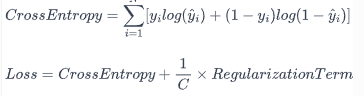
로지스틱 회귀모델에서 모델의 복잡성과 정규화 사이의 균형을 조정하는 중요한 역할을 하는 것은 C값입니다.
C는 정규화의 강도를 조절하는데, 이는 정규화 항의 역수로 정의됩니다.
모델의 손실 함수는 크게 두 부분으로 구성되는데, 하나는 예측값과 실제값의 차이를 나타내는 교차 엔트로피 부분이고, 다른 하나는 모델의 복잡성에 대한 패널티를 부과하는 정규화 항입니다.
import numpy as np
from sklearn.model_selection import KFold, cross_val_score

# K-Fold 교차 검증 설정
kf = KFold(n_splits=5, shuffle=True, random_state=40)

# C 값의 후보 리스트
c_list = [10e-7, 10e-6, 10e-5, 10e-4, 10e-3, 10e-2, 10e-1, 1, 10, 10^2]
scores_list = []

# 각 C에 대한 교차 검증 수행
for c_val in c_list:
    # 로지스틱 회귀 모델 객체 정의, C 값 설정
    logreg_model = LogisticRegression(C=c_val, solver='liblinear', random_state=42)
    # 교차검증, 분류 문제이므로 'accuracy'를 사용
    scores = cross_val_score(logreg_model, X_train, y_train, scoring='accuracy', cv=kf)
    # 평균 점수 저장
    scores_list.append(np.mean(scores))

print('모델의 성능: ', scores_list)

# 최적 alpha 값 및 성능 확인
best_score = max(scores_list) # scores_list에서 최고득점
print(f"Best Score: {best_score}")

optimal_c = c_list[np.argmax(scores_list)] # 최고득점에서의 C의 값
print(f"Optimal C: {optimal_c}")
모델의 성능: [0.7749999999999999, 0.7825, 0.81125, 0.86, 0.8949999999999999, 0.9025000000000001, 0.89375, 0.89375, 0.8925000000000001, 0.8925000000000001]Best Score: 0.9025000000000001
Optimal C: 0.1
1.3 C값의 변화에 따른 모델의 성능 시각화
import matplotlib.pyplot as plt

# 결과 시각화
plt.figure(figsize=(10,6))
plt.plot(c_list, scores_list, marker='o', linestyle='--')
plt.xlabel('C')
plt.ylabel('Cross-Validation Score (Accuacy)')
plt.title('C vs. Accuacy Score')
plt.xscale('log')
plt.show()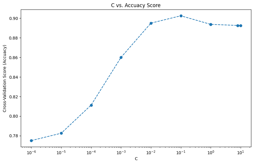
'머신러닝 > 머신러닝: 심화 내용' 카테고리의 다른 글
| 피처 생성(Feature Generation) 2 : 다항식 피처 생성 (0) | 2024.12.24 |
|---|---|
| 피처 생성(Feature Generation) 1 : Binning 기법 (0) | 2024.12.23 |
| 회귀 모델 하이퍼파라미터 튜닝 (0) | 2024.12.20 |
| 교차검증 (1) | 2024.12.19 |
| 차원 축소 기법 : LDA (1) | 2024.12.18 |