1. 카이제곱 통계 분석 및 시각화
교차 테이블을 생성하여 데이터를 정리하고, 이를 기반으로 카이제곱 통계량과 p-값을 계산할 것입니다.
1) 카이제곱 검정의 기본 개념
카이제곱 검정은 범주형 변수 간의 독립성을 평가하기 위한 통계적 방법으로, 두 변수 간의 관계가 우연히 발생한 것인지 아니면 유의미한 관련성이 있는지 확인합니다.
2) 언제 카이제곱 검정을 사용해야 하는가?
범주형 데이터 간의 관계를 이해하고자 할 때 사용됩니다. 예를 들어, 두 범주형 변수 간에 연관성이 있는지를 확인하거나, 범주형 변수의 분포를 비교하고자 할 때 유용합니다.
3) 교차 테이블 생성
교차 테이블은 두 범주형 변수 간의 관계를 요약하는 방법으로, 각 변수별 관측치를 포함하며 이를 통해 두 변수 간의 연관성을 파악할 수 있습니다. Pandas의 crosstab 함수를 사용하여 두 범주형 변수의 빈도수를 계산하여 교차 테이블을 생성할 수 있습니다.
4) p-value
카이제곱 통계량에 대한 p-값은 검정 통계량이 관측된 값보다 더 극단적인 값을 가질 확률을 나타냅니다.
p-값이 특정 유의 수준(예: 0.05)보다 낮다면, 두 변수 사이에는 통계적으로 유의미한 관계가 있다고 결론지을 수 있습니다.
from scipy.stats import chi2_contingency

def chi2_plot(data, column1, column2):
    cross_tab = pd.crosstab(data[column1], data[column2])
    chi2_statistic, p_value, _, _ = chi2_contingency(cross_tab)
    return cross_tab, chi2_statistic, p_value
2. 교육 수준(eduaction)과 타겟(target) 간 카이제곱 검정 및 시각화
cross_tab, chi2_statistic, p_value = chi2_plot(eda_data, 'education', 'target')
print(f'카이제곱 통계량: {chi2_statistic:.2f}')
print(f'p-값: {p_value}')
alpha = 0.05
if p_value < alpha:
print('귀무가설 기각: 두 변수는 통계적으로 독립적이지 않습니다.')
else:
print('귀무가설 채택: 두 변수는 통계적으로 독립적일 가능성이 있습니다.')
# 비율 테이블 생성
ratio_table = cross_tab.div(cross_tab.sum(axis=1), axis='index')
ratio_table_sorted = ratio_table.sort_values(by=0)
# 막대 그래프 그리기
axs = ratio_table_sorted.plot(kind='bar', stacked=True)
axs.set_ylabel('target')
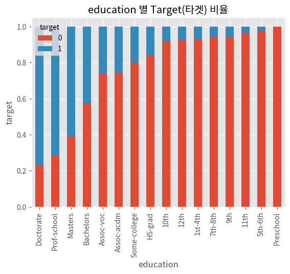
axs.set_title('education 별 Target(타겟) 비율')
plt.show()카이제곱 통계량: 650.21
p-값: 7.476656551203601e-129
귀무가설 기각: 두 변수는 통계적으로 독립적이지 않습니다.
※ 결과 해석
1) 카이제곱 통계량과 p-value
- 카이제곱 통계량은 650.210이고, p-value는 매우 작은 값입니다 (7.48 * e^-129).
- p-value가 0.05보다 작기 때문에 귀무가설을 기각합니다. 이는 education과 target 사이에 통계적으로 유의한 관계가 있음을 의미합니다.
2) 시각화 해석
- Bar(막대) 차트는 각 교육 수준에 따른 target의 분포를 보여줍니다.
- 일부 교육 수준에서 target의 분포는 다른 교육 수준과 상당히 다르게 나타납니다. 예를 들어, HS-grad와 Some-college 카테고리는 target 값이 0인 비율이 높은 반면, Doctorate와 Prof-school 카테고리는 target 값이 1인 비율이 높습니다.
- 교육 수준(education)은 target 변수에 영향을 미치는 것으로 보입니다. 높은 교육 수준을 가진 사람들은 높은 target 값을 가질 가능성이 높습니다.
- 이 분석은 교육 수준이 target 값에 영향을 미칠 수 있음을 나타내므로, 이 변수는 모델링에서 사용될 중요한 특성일 수 있습니다.
3. 교육 수준(education) 범주화 후의 카이제곱 검정 비교
eda_data['education'].replace(['Doctorate', 'Prof-school'], 'Advanced', inplace=True)
eda_data['education'].replace(['Assoc-acdm', 'Assoc-voc'], 'Intermediate', inplace=True)
eda_data['education'].replace(['Preschool', '10th', '11th', '12th', '1st-4th', '5th-6th', '7th-8th', '9th'], 'Basic', inplace=True)

###
_, chi2_statistic, p_value = chi2_plot(eda_data, 'education', 'target')

print(f'카이제곱 통계량: {chi2_statistic:.2f}')
print(f'p-값: {p_value}')

alpha = 0.05
if p_value < alpha:
    print('귀무가설 기각: 두 변수는 통계적으로 독립적이지 않습니다.')
else:
    print('귀무가설 채택: 두 변수는 통계적으로 독립적일 가능성이 있습니다.')
카이제곱 통계량: 648.27
p-값: 8.997515603957002e-137
귀무가설 기각: 두 변수는 통계적으로 독립적이지 않습니다.※ 결과 해석
- 독립성 여부: 두 경우 모두 귀무가설이 기각되었습니다. 이는 education과 target 변수가 통계적으로 독립적이지 않다는 것을 의미합니다. 즉, 이 두 변수 사이에는 어떤 관련성이 존재합니다.
- 범주화의 영향: 범주화 전과 후의 카이제곱 통계량과 p-값에는 미세한 차이가 있습니다. 범주화 후 p-값이 더 작아졌으며, 이는 두 변수 간의 관련성이 더 강하게 나타난다는 것을 의미할 수 있습니다. 범주화를 통해 데이터의 구조가 단순화되었고, 이는 변수 간 관계를 더 명확하게 드러낼 수 있습니다.
- 통계적 유의성: 두 경우 모두 매우 작은 p-값을 가지고 있으며, 이는 두 변수 간의 관계가 매우 강한 통계적 유의성을 가짐을 나타냅니다. 특히 범주화 후 p-값이 더 낮아져, 교육 수준과 소득 수준 간의 관계가 더욱 뚜렷하게 나타나는 것으로 해석될 수 있습니다.
- 데이터 분석의 통찰: 이 결과는 교육 수준이 소득 수준과 어떤 관련이 있음을 시사합니다. 즉, 교육 수준이 높을수록 더 높은 소득 수준을 가질 가능성이 크다고 해석할 수 있습니다. 이러한 인사이트는 교육과 소득 수준 간의 관계를 더 깊이 이해하는 데 도움이 될 수 있습니다.
4. 본 국적(native.country) 시각화
country_data = eda_data.dropna(subset=['native.country'])

fig, ax = plt.subplots(figsize=(8, 5))
sns.countplot(y='native.country', data=country_data, ax=ax)

ax.set_title('Distribution of Native Countries')
ax.set_xlabel('Count')
ax.set_ylabel('Native Country')

plt.tight_layout()
plt.show()
※ 결과 해석
그래프를 통해 대다수 사람들이 미국(United-States) 출신임을 확인할 수 있습니다. 이로 보아 이 데이터셋은 주로 미국 인구에 초점을 맞춘 것으로 보입니다. 미국 외 다른 국가들은 상대적으로 적은 관측값을 보유하고 있습니다. 이는 이러한 국가들의 데이터가 데이터셋에서 큰 부분을 차지하지 않음을 의미합니다. 다양한 국가의 데이터가 있지만, 그 분포는 매우 불균형합니다. 미국 이외의 대부분 국가들은 데이터셋에서 매우 작은 비중을 차지하고 있습니다.
5. 본 국적(native.country)과 타겟(target) 간 카이제곱 검정 및 시각화
cross_tab, chi2_statistic, p_value = chi2_plot(eda_data, 'native.country', 'target')

print(f'카이제곱 통계량: {chi2_statistic:.2f}')
print(f'p-값: {p_value}')

alpha = 0.05
if p_value < alpha:
    print('귀무가설 기각: 두 변수는 통계적으로 독립적이지 않습니다.')
else:
    print('귀무가설 채택: 두 변수는 통계적으로 독립적일 가능성이 있습니다.')

# 비율 테이블 생성
ratio_table = cross_tab.div(cross_tab.sum(axis=1), axis='index')
ratio_table_sorted = ratio_table.sort_values(by=0)

# 막대 그래프 그리기
axs = ratio_table_sorted.plot(kind='bar', stacked=True)
axs.set_xlabel('native.country')
axs.set_ylabel('target')
axs.set_title('native.country 별 Target(타겟) 비율')
plt.show()
카이제곱 통계량: 67.05
p-값: 0.0034516485374650268
귀무가설 기각: 두 변수는 통계적으로 독립적이지 않습니다.
※ 결과 해석
p-value가 0.05보다 작으므로 귀무가설을 기각하게 됩니다. 이는 국가별 출신 인구와 소득 수준 사이에는 통계적으로 유의미한 관계가 있다는 것을 의미합니다.
바 그래프를 통해 각 국가별로 소득이 50K 이상인 인구의 비율을 살펴보았습니다. 그 결과, 일부 국가에서는 높은 소득을 가진 인구의 비율이 더 높았고, 일부 국가에서는 그렇지 않았습니다.
이러한 결과는 각 국가의 경제 상태, 교육 수준, 직업 기회 등 다양한 외부 요인에 영향을 받을 수 있습니다. 또한, 데이터 내의 국가별 샘플 수의 차이도 결과에 영향을 줄 수 있으며, 일부 국가의 경우 샘플 수가 적어 분석 결과의 신뢰성이 떨어질 수 있습니다.
6. 국가(native.country)별 타겟(target) 비율에 따른 본 국적 범주화(그룹화)
다양한 국가의 데이터가 있지만, 그 분포는 매우 불균형한 점 을 고려하여 proportion 값을 기준으로 교육 수준을 5개의 그룹 중 하나로 분리 하겠습니다.
A_group = []
B_group = []
C_group = []
D_group = []
E_group = []

for country_level in eda_data['native.country'].unique():
    education_data = eda_data[eda_data['native.country'] == country_level]['target']
    proportion = sum(education_data) / education_data.count()

    if proportion == 0.0:
        A_group.append(country_level)
    elif proportion > 0.0 and proportion <=0.2:
        B_group.append(country_level)
    elif proportion > 0.2 and proportion <=0.4:
        C_group.append(country_level)
    elif proportion > 0.4 and proportion <=0.6:
        D_group.append(country_level)
    else:
        E_group.append(country_level)

print('Group 1 (Proportion == 0.0):', A_group)
print('Group 2 (0.0 < Proportion <= 0.2):', B_group)
print('Group 3 (0.2 < Proportion <= 0.4):', C_group)
print('Group 4 (0.4 < Proportion <= 0.6):', D_group)
print('Group 5 (Proportion > 0.6):', E_group)
Group 1 (Proportion == 0.0): ['Guatemala', 'Puerto-Rico', 'Jamaica', 'Thailand', 'Portugal', 'Poland', 'Haiti', 'Vietnam', 'Honduras', 'Laos', 'Yugoslavia', 'Peru', 'Nicaragua', 'Outlying-US(Guam-USVI-etc)', 'Hong', 'Scotland']
Group 2 (0.0 < Proportion <= 0.2): ['Mexico', 'Columbia', 'China', 'Philippines', 'Taiwan', 'Germany', 'Dominican-Republic', 'France', 'El-Salvador', 'Cuba']
Group 3 (0.2 < Proportion <= 0.4): ['United-States', 'Trinadad&Tobago', 'India', 'England', 'South', 'Ecuador', 'Italy']
Group 4 (0.4 < Proportion <= 0.6): ['Canada', 'Japan', 'Ireland', 'Hungary', 'Cambodia', 'Greece']
Group 5 (Proportion > 0.6): [nan, 'Iran']
7. 국가(native.country)별 타겟(target) 비율에 따른 본 국적 범주화(그룹화) 적용
eda_data['native.country']=eda_data['native.country'].replace(A_group,0)
eda_data['native.country']=eda_data['native.country'].replace(B_group,1)
eda_data['native.country']=eda_data['native.country'].replace(C_group,2)
eda_data['native.country']=eda_data['native.country'].replace(D_group,3)
eda_data['native.country']=eda_data['native.country'].replace(E_group,4)

###
cross_tab, chi2_statistic, p_value = chi2_plot(eda_data, 'native.country', 'target')

print(f'카이제곱 통계량: {chi2_statistic:.2f}')
print(f'p-값: {p_value}')

alpha = 0.05
if p_value < alpha:
    print('귀무가설 기각: 두 변수는 통계적으로 독립적이지 않습니다.')
else:
    print('귀무가설 채택: 두 변수는 통계적으로 독립적일 가능성이 있습니다.')
카이제곱 통계량: 52.26
p-값: 1.2181355132417364e-10
귀무가설 기각: 두 변수는 통계적으로 독립적이지 않습니다.※ 결과 해석
1) 관계의 강도
범주화 전과 후 모두 귀무가설이 기각되어 두 변수 간에는 통계적으로 유의미한 관련성이 있음을 나타냅니다. 하지만 카이제곱 통계량이 범주화 후에 낮아졌습니다. 이는 범주화를 통해 native.country와 target 간의 관계가 덜 명확해졌을 수 있음을 시사합니다.
2) p-값의 변화
범주화 후 p-값이 더 작아졌습니다. 이는 범주화를 통해 두 변수 간의 관계가 더 강한 통계적 유의성을 가짐을 나타냅니다. 다시 말해, 범주화를 통해 변수 간의 관련성이 더 명확하게 드러나게 되었습니다.
3) 데이터의 해석 가능성
범주화 후 데이터는 해석하기 더 간단해질 수 있습니다. 원래 많은 국가들이 각기 다른 비율을 가지고 있었지만, 범주화를 통해 이를 명확한 그룹으로 나누어 데이터를 더 쉽게 해석하고 분석할 수 있게 되었습니다.
4) 모델링의 영향
이러한 범주화는 머신러닝 모델링에서 변수의 중요도를 평가하거나, 변수 간의 상호작용을 이해하는 데 도움이 될 수 있습니다. 단순화된 범주화를 통해 모델이 더 강한 패턴을 학습할 수 있을 것입니다.
5) Feature Engineering
모델의 예측 능력을 향상시키는 방법으로 변수 사이의 관계를 개선한 것만으로도 데이터의 최적화로 인해 모델의 성능 향상을 기대할 수 있습니다. 하지만 이러한 과정을 실제 예측 모델에서 성능 평가를 통해 확인해야 합니다.
8. 나이(age)와 주당 근로시간(hours.per.week) 관계 분석
sns.jointplot(data=eda_data, x="age", y="hours.per.week", hue="target")
plt.show()
※ 결과 해석
1) 분포 밀도
대부분의 데이터 포인트는 나이가 낮고 주당 근무 시간이 중간 정도인 영역에 집중되어 있습니다.
고소득 그룹(target=1)은 주로 중간 나이대와 높은 주당 근무 시간에 분포해 있는 것으로 보입니다.
2) 상관 관계
나이와 주당 근무 시간 간에는 뚜렷한 상관 관계가 보이지 않습니다. 하지만, 고소득 그룹에서는 나이가 많고 주당 근무 시간이 높은 경우가 다소 많은 것으로 보입니다.
3) target에 따른 분포
고소득 그룹은 나이가 높고, 주당 근무 시간이 많은 구간에 비교적 많이 분포하고 있습니다.
저소득 그룹은 넓게 분포해 있으며, 특히 젊은 나이 대에서 많이 볼 수 있습니다.
9. age feture 범주화
eda_data['age_bin'] = pd.cut(eda_data['age'], 30)

fig, axs = plt.subplots(1, 2, figsize=(20, 5))

# 첫 번째 서브플롯: 나이별 빈도수
sns.countplot(x="age_bin", data=eda_data, ax=axs[0])
axs[0].set_xticklabels(axs[0].get_xticklabels(), rotation=45)

# 두 번째 서브플롯: 나이 분포 비교
sns.distplot(eda_data[eda_data['target'] == 1]['age'], kde_kws={"label": ">$50K"}, ax=axs[1])
sns.distplot(eda_data[eda_data['target'] == 0]['age'], kde_kws={"label": "<=$50K"}, ax=axs[1])

plt.tight_layout()
plt.show()
※ 결과 해석
1) 첫 번째 서브플롯 (나이별 빈도수)
이 차트에서는 나이를 30개 구간으로 나누어 각 구간별 빈도수를 보여줍니다. 이를 통해 데이터셋 내에서 다양한 연령대의 분포를 파악할 수 있습니다.
특정 연령대, 예를 들어 20대 중반에서 30대 초반 사이의 구간에서 높은 빈도수를 관찰할 수 있습니다. 이는 데이터셋에 젊은 연령대가 많이 포함되어 있음을 나타냅니다.
반면, 매우 젊은 연령대(예: 10대)나 고령자(예: 70대 이상)의 빈도수는 상대적으로 낮음을 볼 수 있습니다. 이는 데이터셋에서 이러한 연령대의 인구 비율이 낮음을 시사합니다.
2) 두 번째 서브플롯 (나이 분포 비교)
두 번째 차트는 소득 수준(target)에 따른 나이 분포를 비교합니다. 여기서 두 개의 분포 곡선(소득이 $50K 이상 그룹과 $50K 이하 그룹)을 통해 소득 수준에 따라 나이 분포가 어떻게 다른지 비교할 수 있습니다.
소득이 $50K 이상인 그룹에서는 중년층의 분포가 두드러지게 나타납니다. 이는 중년층이 소득의 증가를 경험할 가능성이 높음을 나타내며, 경력과 경험이 소득에 중요한 역할을 할 수 있음을 시사합니다.
반면, 소득이 $50K 이하인 그룹에서는 젊은 연령대의 분포가 높게 나타납니다. 이는 경력이 적은 연령대에서 낮은 소득 수준을 가진 사람들이 더 많이 분포함을 나타냅니다.
10. train 데이터에 범주화(교육 수준(education), 결혼 상태(marital.status), 본 국적(native.country)) 적용
def categorize_features(data):
    # Education 범주화
    data['education'].replace(['Doctorate', 'Prof-school'], 'Advanced', inplace=True)
    data['education'].replace(['Assoc-acdm', 'Assoc-voc'], 'Intermediate', inplace=True)
    data['education'].replace(['Preschool', '10th', '11th', '12th', '1st-4th', '5th-6th', '7th-8th', '9th'], 'Basic', inplace=True)

    # Marital Status 범주화
    data['marital.status'].replace(['Never-married', 'Married-spouse-absent'], 'UnmarriedStatus', inplace=True)
    data['marital.status'].replace(['Married-AF-spouse', 'Married-civ-spouse'], 'Married', inplace=True)
    data['marital.status'].replace(['Separated', 'Divorced'], 'MarriageEnded', inplace=True)

    # Native Country 범주화
    data['native.country'] = data['native.country'].replace(A_group, 0)
    data['native.country'] = data['native.country'].replace(B_group, 1)
    data['native.country'] = data['native.country'].replace(C_group, 2)
    data['native.country'] = data['native.country'].replace(D_group, 3)
    data['native.country'] = data['native.country'].replace(E_group, 4)

    return data
11. 파생 변수 생성: 나이(age)와 주당 근무 시간(hours.per.week)의 곱, 나이(age) 범주화
def create_age_hours_feature(data):
    data['age-hours'] = data['age'] * data['hours.per.week']
    data['age'] = pd.cut(np.log(data['age']), 30)
    return data
※ age와 hours.per.week 피처를 곱한 파생변수의 장점
1) 상호작용 효과 포착
연령과 주당 근무시간의 곱은 두 변수 간의 상호작용 효과를 나타냅니다. 예를 들어, 같은 수의 근무시간을 가진 두 사람이더라도 연령에 따라 실제 노동 생산성이 다를 수 있습니다. 이러한 상호작용을 모델이 포착할 수 있도록 도와줍니다.
2) 비선형 관계 모델링
많은 기계 학습 모델들은 기본적으로 변수들 사이의 선형 관계를 학습합니다. 변수들을 곱하여 새로운 특성을 만들어내면, 모델이 이러한 비선형 관계를 더 잘 이해하고 포착할 수 있습니다.
3) 특성의 중요성 강조
두 변수를 곱함으로써 어떤 변수가 각기 변수에 더 큰 영향을 미치는지를 모델에 더 명시적으로 나타낼 수 있습니다. 이는 특히 교차항이 중요한 역할을 할 때 유용합니다.
※ age 변수를 로그 변환 후 30개의 범주로 범주화하는 것의 장점
1)연령대별 특성 파악
나이를 범주화하면, 각 연령대로 데이터가 어떻게 분포되어 있는지 더 명확하게 이해할 수 있습니다. 이는 연령대별 특성과 소득 수준 간의 관계를 분석하는 데 유용합니다.
2)파생 변수 생성
pd.cut 함수를 사용하여 나이를 범주화함으로써, 나이를 연령대별 구간으로 나누어 새로운 파생 변수를 생성할 수 있습니다. 이러한 변수를 통해 모델의 성능을 향상시킬 수 있는 중요한 입력 값이 될 가능성이 큽니다.
3)모델의 해석 용이성
나이를 범주화하면, 모델이 나이와 소득 수준 간의 관계를 더 쉽게 학습하고 해석할 수 있습니다. 특히, 이해관계자나, 런던 표시로 통의 문제에서 범주화된 변수는 중요한 분석 기준이 될 수 있습니다.
12. 랜덤포레스트를 활용한 직업(occupation) 결측치 대체
from sklearn.ensemble import RandomForestClassifier

def impute_missing_occupation(train_data):

    missing_occupation = train_data[train_data['occupation'].isnull()]
    non_missing_occupation = train_data[~train_data['occupation'].isnull()] # 결측값이 없는 행

    missing_occupation = missing_occupation.copy()
    non_missing_occupation = non_missing_occupation.copy() # 원본 데이터를 손상시키지않기 위해 복사본 생성

    non_missing_occupation['occupation'] = non_missing_occupation['occupation'].astype('category') # 'occupation' 열을 카테고리 타입으로 변환
    occupation_categories = non_missing_occupation['occupation'].cat.categories # occupation 피처의 고유한 카테고리 목록을 추출
    category_to_number = {category: number for number, category in enumerate(occupation_categories)} # occupation_categories 목록의 각 카테고리에 번호를 할당한 딕셔너리를 생성
    non_missing_occupation['occupation'] = non_missing_occupation['occupation'].map(category_to_number) # 각 카테고리를 해당 번호로 인코딩

    numeric_columns = non_missing_occupation.select_dtypes(include=['int64', 'float64']).columns.tolist() + ['occupation'] # 수치형 데이터 열의 이름을 리스트 형태로 반환, 리스트에 occupation 열을 추가

    x_train = non_missing_occupation[numeric_columns[:-1]]
    y_train = non_missing_occupation[numeric_columns[-1]] # 종속변수만 선택한 후 y_train 변수에 할당
    x_valid = missing_occupation[numeric_columns[:-1]]

    model = RandomForestClassifier(random_state=24) # RandomForestClassifier 모델을 생성, random_state를 24로 설정하여 재현성을 보장
    model.fit(x_train, y_train) # 모델 학습
    predicted_occupation = model.predict(x_valid) # 모델 예측
    missing_occupation['occupation'] = predicted_occupation # 결측값 대체

    train_imputed_occupation = pd.concat([non_missing_occupation, missing_occupation]) # 결측값이 없는 데이터와 결측값을 대체한 데이터 합치기
    number_to_category = {num: cat for cat, num in category_to_number.items()} # 카테고리 매핑 역방향 설정
    train_imputed_occupation['occupation'] = train_imputed_occupation['occupation'].map(number_to_category) # 'occupation' 열을 카테고리로 복원

    return train_imputed_occupation
13. 학습 및 테스트 데이터의 결측값 대체
from sklearn.impute import SimpleImputer
from sklearn.preprocessing import LabelEncoder

def impute_missing_values(train, valid, columns_to_impute):
    imputed_train_data = train.copy()
    imputed_valid_data = valid.copy()

    imputer = SimpleImputer(strategy='most_frequent')
    imputed_train_data[columns_to_impute] = imputer.fit_transform(imputed_train_data[columns_to_impute])
    imputed_valid_data[columns_to_impute] = imputer.transform(imputed_valid_data[columns_to_impute])

    return imputed_train_data, imputed_valid_data

def label_encoding(train_data, test_data):
    select_category_columns = train_data.select_dtypes(['object', 'category']).columns
    target = ['ID', 'target']  # 제외하고자 하는 열 이름
    result = [x for x in select_category_columns if x not in target]

    for col in result:
        if train_data[col].dtype == 'object' or train_data[col].dtype == 'category':
            le = LabelEncoder()
            train_data[col] = le.fit_transform(train_data[col])

            for label in np.unique(test_data[col]):
                if label not in le.classes_:
                    le.classes_ = np.append(le.classes_, label)
            test_data[col] = le.transform(test_data[col])
    return train_data, test_data
14. 데이터 전처리 및 특성 엔지니어링 함수 적용
train_origin = pd.read_csv('train.csv')

categorize_three_features = categorize_features(train_origin)
create_age_hours = create_age_hours_feature(categorize_three_features)

from sklearn.model_selection import train_test_split
train_data, valid_data = train_test_split(create_age_hours, test_size=0.2, random_state=42, stratify=train_origin['target'])
imputed_train_occupation = impute_missing_occupation(train_data)

columns_to_impute = ['occupation', 'workclass', 'native.country']
imputed_train_data, imputed_valid_data = impute_missing_values(imputed_train_occupation, valid_data, columns_to_impute)
encoded_train, encoded_valid = label_encoding(imputed_train_data, imputed_valid_data)
15. 로그 변환(Log1p)을 적용한 모델 훈련 및 평가
from sklearn.metrics import make_scorer, f1_score
from sklearn.model_selection import cross_val_score

L_encoded_train = encoded_train.copy()
L_encoded_valid = encoded_valid.copy()

L_encoded_train['log1p_loss'] = np.log1p(L_encoded_train['capital.loss'])
L_encoded_train['log1p_gain'] = np.log1p(L_encoded_train['capital.gain'])

L_encoded_valid['log1p_loss'] = np.log1p(L_encoded_valid['capital.loss'])
L_encoded_valid['log1p_gain'] = np.log1p(L_encoded_valid['capital.gain'])

train_y = L_encoded_train['target']
train_x = L_encoded_train.drop(['ID','target','capital.gain','capital.loss','education.num'],axis = 1)

valid_y = L_encoded_valid['target']
valid_x = L_encoded_valid.drop(['ID','target','capital.gain','capital.loss','education.num'],axis = 1)

from sklearn.ensemble import ExtraTreesClassifier

extra = ExtraTreesClassifier(random_state=24)
f1_scorer = make_scorer(f1_score, average='macro')
cross_val_scores = cross_val_score(extra, train_x, train_y, cv=3, scoring=f1_scorer)
mean_f1_score = np.mean(cross_val_scores)
print("Mean Cross-Validation F1 Score:", mean_f1_score)
Mean Cross-Validation F1 Score: 0.7727553343966492※ 결과 해석
log1p 변환은 주로 데이터의 스케일을 조정하고, 큰 값을 가진 이상치의 영향을 줄이기 위해 사용됩니다.
capital.loss와 capital.gain 특성에 log1p 변환을 적용하여, 이들 특성이 값이 매우 큰 범위를 가질 때 이를 완화합니다.
이 방법은 데이터의 전반적인 분포를 더 정규 분포에 가깝게 만들어 줄 수 있으며, 모델이 데이터를 더 잘 이해하고 학습하는 데 도움을 줍니다.
log1p 변환 후의 F1 스코어는 0.7716입니다. 이는 변환을 통해 데이터의 정규성을 향상시키면서 분류 성능을 어느 정도 개선했음을 보여줍니다. 모델이 데이터를 분류하는 데 있어서 상대적으로 보통 수준의 성능을 보여줍니다.
16. DASCAN을 적용한 모델 훈련 및 평가
from sklearn.cluster import DBSCAN

D_encoded_train = encoded_train.copy()
D_encoded_valid = encoded_valid.copy()

X_sample_scaled = D_encoded_train[['capital.gain', 'capital.loss']]

dbscan = DBSCAN(eps=0.5, min_samples=4)
clusters_sample = dbscan.fit_predict(X_sample_scaled)

D_encoded_train['clusters'] = clusters_sample
sample_no_outliers = D_encoded_train[D_encoded_train['clusters'] != -1]

train_y = sample_no_outliers['target']
train_x = sample_no_outliers.drop(['ID','target','education.num','clusters'],axis = 1)

valid_y = D_encoded_valid['target']
valid_x = D_encoded_valid.drop(['ID','target','education.num'],axis = 1)

from sklearn.ensemble import ExtraTreesClassifier

extra = ExtraTreesClassifier(random_state=24)
f1_scorer = make_scorer(f1_score, average='macro')
cross_val_scores = cross_val_score(extra, train_x, train_y, cv=3, scoring=f1_scorer)
mean_f1_score = np.mean(cross_val_scores)
print("Mean Cross-Validation F1 Score:", mean_f1_score)
Mean Cross-Validation F1 Score: 0.7843746695473008※ 결과 해석
DBSCAN은 밀도 기반의 클러스터링 알고리즘으로, 데이터의 밀도가 낮은 부분을 이상치로 간주하여 제거합니다.
capital.gain과 capital.loss 특성에 DBSCAN을 적용하여, 이상치로 간주되는 데이터 포인트를 식별하고 제거합니다.
이 방법은 실제로 이상치를 데이터셋에서 제거함으로써, 모델이 주요 데이터 패턴에 더 집중할 수 있도록 합니다.
DBSCAN을 적용한 후의 F1 스코어는 0.7872로, 이는 log1p 변환을 사용했을 때보다 더 높은 성능을 나타냅니다.
이는 DBSCAN이 데이터셋에서 이상치를 효과적으로 제거하여 모델이 더 정확하게 데이터를 학습할 수 있게 만들었음을 시사합니다.
'머신러닝 > 머신러닝: 실전 프로젝트 학습' 카테고리의 다른 글
| 인구 소득 예측 프로젝트 6 : 종합적 데이터 처리와 고급 모델 튜닝을 통한 성능 향상 (0) | 2025.01.02 |
|---|---|
| 인구 소득 예측 프로젝트 5 : 클래스 불균형(Borderline SMOTE)과 정규화(StandardScaler)를 활용한 모델 성능 최적화 (0) | 2025.01.01 |
| 인구 소득 예측 프로젝트 3 : 이상치 처리 (0) | 2024.12.31 |
| 인구 소득 예측 프로젝트 2 : 결측값 처리 (1) | 2024.12.31 |
| 인구 소득 예측 프로젝트 1 : 데이터 분석 (1) | 2024.12.30 |