1. 심층(Staked) LSTM
1) 개요
Stacked LSTM은 여러 개의 LSTM 층을 쌓아올린 심층 구조의 LSTM 모델입니다.
기본적인 LSTM은 단일 층으로 이루어져 있지만, Stacked LSTM은 여러 개의 LSTM 층을 수직으로 쌓아 심층 구조를 형성합니다.
각 LSTM 층의 출력이 다음 층의 입력으로 전달되며, 이를 통해 더욱 복잡하고 추상적인 특징을 학습할 수 있습니다.
이는 모델이 입력 데이터를 더욱 효과적으로 처리하고, 다양한 패턴을 포착할 수 있게 해줍니다.
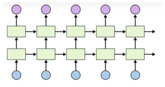
※ Stacked LSTM의 구조
Stacked LSTM의 구조는 다음과 같습니다.
각 시점의 입력 데이터는 첫 번째 LSTM 층으로 전달됩니다.
첫 번째 층의 출력은 두 번째 LSTM 층의 입력으로 사용되며, 이러한 방식으로 최종 LSTM 층까지 전달됩니다.
마지막 LSTM 층의 출력이 최종 모델의 출력으로 사용됩니다.
이 다층 구조는 입력 데이터의 점진적인 추상화와 복잡한 패턴 인식을 가능하게 합니다.
※ Stacked LSTM은 언제, 왜 사용하는가
Stacked LSTM은 단일 LSTM보다 더 깊은 구조를 가지고 있어 복잡한 패턴과 장기 의존성을 더 잘 포착할 수 있습니다. 그러나 이는 모든 경우에 적절한 것은 아닙니다. 다음과 같은 상황에서 Stacked LSTM이 특히 유용할 수 있습니다.
- 시계열 데이터 예측
장기간의 트렌드와 변동을 포착하는 데 유리합니다.
그러나 데이터의 복잡성이 낮다면 단일 LSTM도 충분히 좋은 성능을 발휘할 수 있습니다. - 자연어 처리(NLP)
문장의 문맥과 의미를 더 깊이 이해할 수 있습니다.
하지만, 간단한 문장 구조나 단기 의존성이 중요한 경우 단일 LSTM이 더 적합할 수 있습니다. - 음성 인식
긴 음성 데이터를 처리하여 더 정확한 인식을 수행할 수 있습니다.
하지만 데이터가 짧고 평균 길다면 단일 LSTM도 충분할 수 있습니다.
Stacked LSTM을 사용하면 단일 층 LSTM보다 더 높은 성능을 얻을 수 있으며, 모델의 표현력과 학습 능력을 향상시킬 수 있습니다. 이를 통해 보다 긴 시퀀스 기반 문제에서 우수한 성능을 기대할 수 있지만, 항상 모델이 향상되는 것은 아니라는 점을 염두에 두어야 합니다.
※ Stacked LSTM의 한계점
- 계산 비용 증가:
더 많은 층을 사용하면 계산 비용이 증가하고, 학습 시간이 더 오래 걸릴 수 있습니다. - 과적합 위험:
모델이 너무 복잡해지면 학습 데이터에 과적합할 가능성이 높아집니다. - 하이퍼파라미터 튜닝 필요:
층 수가 늘어날수록 하이퍼파라미터를 적절히 설정해야 최적의 성능을 확보할 수 있습니다.
2) 이전 스테이지 코드 불러오기 및 함수 파일 활용
import pandas as pd
df_weather_org = pd.read_csv('sample_weather_data.csv')
features = ['humidity','rainfall','wspeed','temperature']
target_col = ['temperature']

display(f"데이터 갯수 : {len(df_weather_org)}")
display(df_weather_org.head())

from LSTM_stage2 import *

#####################################################################################################
# 아래 코드는 이전에 정의한 함수들을 확인하기 위한 코드 입니다. 학습해야 할 내용과는 직접 관련이 없습니다.
#####################################################################################################

import inspect
print(inspect.getsource(set_seed).splitlines()[0])
print(inspect.getsource(build_sequence_dataset).splitlines()[0])
print(inspect.getsource(train).splitlines()[0])
print(inspect.getsource(validate_model).splitlines()[0])
print(inspect.getsource(sliding_window_split).splitlines()[0])
print(inspect.getsource(plot_results).splitlines()[0])
'데이터 갯수 : 730'| 2021-01-01 | 64.0 | 0.0 | 2.0 | -4.2 |
| 2021-01-02 | 38.5 | 0.0 | 2.6 | -5.0 |
| 2021-01-03 | 45.0 | 0.0 | 2.0 | -5.6 |
| 2021-01-04 | 51.4 | 0.0 | 1.7 | -3.5 |
| 2021-01-05 | 52.8 | 0.0 | 2.9 | -5.5 |
def set_seed(seed_value):
def build_sequence_dataset(df, taget, seq_length):
def train(model, train_loader, optimizer, criterion):
def validate_model(model, test_loader, criterion):
def sliding_window_split(data, train_size, test_size, seq_length):
def plot_results(train_loss_lst, test_loss_lst, actuals, predictions, fold=None):
3) nn.LSTM을 이용한 심층(Stacked) LSTM 인스턴스 생성
import torch
import torch.nn as nn

# LSTM 인스턴스 생성
# 'stackedlstm_ex1' 변수명은 정답체크를 위해 수정하지 마세요
stackedlstm_ex1 = nn.LSTM(input_size=5, hidden_size=20, num_layers=2)

print("Input size : {stackedlstm.input_size}")
print(f"stackedlstm.hidden_size : {stackedlstm_ex1.hidden_size}" )
print(f"stackedlstm.hidden_size.shape : {stackedlstm_ex1.num_layers}" )
Input size : {stackedlstm.input_size}
stackedlstm.hidden_size : 20
stackedlstm.hidden_size.shape : 2
※ 결과 해석
위 코드에서는 input_size를 5, hidden_size를 20, num_layers를 2로 설정하여 Stacked LSTM을 생성합니다.
이 설정은 입력 데이터의 특징 수가 5개, 각 LSTM 층의 은닉 상태 크기가 20개이며, 2개의 LSTM 층을 쌓은 모델을 만듭니다.
4) StackedLSTM 클래스 만들기
class StackedLSTM(nn.Module):
def __init__(self, input_size, hidden_size, num_layers, output_size, dropout_rate=0.15):
super(StackedLSTM, self).__init__()
self.hidden_size = hidden_size
self.num_layers = num_layers
self.lstm = nn.LSTM(input_size, hidden_size, num_layers, batch_first=True, dropout = dropout_rate)
self.fc1 = nn.Linear(hidden_size, hidden_size//2)
self.fc2 = nn.Linear(hidden_size//2, output_size)
self.dropout = nn.Dropout(dropout_rate)
self.relu = nn.ReLU()
def forward(self, x):
batch_size = x.size(0)
h0, c0 = self.init_hidden(batch_size, x.device)
out, _ = self.lstm(x, (h0, c0))
out = self.dropout(out[:, -1, :]) # LSTM과 FC1 사이에 Dropout 적용
out = self.fc1(out)
out = self.relu(out)
out = self.fc2(out)
return out
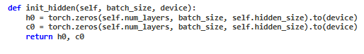
def init_hidden(self, batch_size, device):
h0 = torch.zeros(self.num_layers, batch_size, self.hidden_size).to(device)
c0 = torch.zeros(self.num_layers, batch_size, self.hidden_size).to(device)
return h0, c0
# 'stackedlstm_ex2' 변수명은 정답체크를 위해 수정하지 마세요
stackedlstm_ex2 = StackedLSTM(input_size=5, hidden_size=20, num_layers=2, output_size=1, dropout_rate=0.2)
stackedlstm_ex2StackedLSTM(
(lstm): LSTM(5, 20, num_layers=2, batch_first=True, dropout=0.2)
(fc1): Linear(in_features=20, out_features=10, bias=True)
(fc2): Linear(in_features=10, out_features=1, bias=True)
(dropout): Dropout(p=0.2, inplace=False)
(relu): ReLU()
)
※ 코드 해석
LSTM 레이어: 입력 데이터를 순차적으로 처리하여 시계열 패턴을 학습합니다. input_size는 입력 데이터의 특징 수, hidden_size는 각 LSTM 층의 은닉 상태 크기, num_layers는 LSTM 층의 수를 나타냅니다. dropout은 LSTM 층 사이에서 드롭아웃을 적용하여 과적합을 방지합니다.
self.lstm = nn.LSTM(input_size, hidden_size, num_layers, batch_first=True, dropout=dropout_rate)
Fully Connected (FC) 레이어: LSTM 레이어의 마지막 출력을 받아 최종 예측값을 생성합니다. 두 개의 FC 레이어를 사용하여 모델의 복잡성을 줄이고, 더 추상적인 특징을 학습할 수 있도록 합니다.
self.fc1 = nn.Linear(hidden_size, hidden_size // 2)
self.fc2 = nn.Linear(hidden_size // 2, output_size)
첫 번째 FC 레이어는 hidden_size의 절반 크기를 사용하여 출력 차원을 줄입니다. 이는 모델의 복잡성을 줄이고, 계산 효율성을 높이며, 과적합을 방지하는 데 도움이 됩니다.
두 번째 FC 레이어는 첫 번째 FC 레이어의 출력을 받아 최종 출력 차원으로 변환합니다.
Dropout 레이어: 과적합을 방지하기 위해 일부 뉴런을 무작위로 비활성화합니다. 여기서는 LSTM 레이어와 첫 번째 FC 레이어 사이에 적용하여 LSTM의 출력을 정규화합니다.
self.dropout = nn.Dropout(dropout_rate)
ReLU 활성화 함수: 첫 번째 FC 레이어의 출력에 비선형성을 추가하여 모델의 표현력을 높입니다. ReLU는 계산이 간단하고, 기울기 소실 문제를 완화하는 장점이 있습니다.
self.relu = nn.ReLU()
※ Forward 메서드
LSTM 레이어 출력:
입력 데이터 X를 LSTM 레이어를 통해 처리합니다. 이때, 초기 은닉 상태 h0와 셀 상태 c0를 설정합니다.
h0, c0 = self.init_hidden(batch_size, x.device) out, _ = self.lstm(x, (h0, c0))
Dropout 적용:
LSTM 레이어의 마지막 시점의 출력(out[:, -1, :])에 Dropout을 적용하여 과적합을 방지합니다.
out = self.dropout(out[:, -1, :])
Fully Connected 레이어와 ReLU 적용:
Dropout을 통과한 출력을 첫 번째 FC 레이어로 전달하고,
ReLU 활성화 함수를 적용하여 비선형성을 추가합니다.
out = self.fc1(out)
out = self.relu(out)
최종 출력:
두 번째 FC 레이어를 통해 최종 예측값을 생성합니다.
out = self.fc2(out)
초기 은닉 상태 설정:
init_hidden 메서드는 LSTM 층의 초기 은닉 상태와 셀 상태를 생성합니다.
5) Sliding_window_split 함수 작성
import numpy as np

def sliding_window_split(data, train_size, test_size, seq_length):

    splits = []
    start = len(data) - (train_size + test_size)
    while start >= 0:
        train_index = np.arange(start, start + test_size)
        test_index = np.arange(start + train_size, start + train_size+test_size)
        splits.append((train_index, test_index))
        start -= test_size  # 테스트 데이터 크기만큼 이동
    return splits[::-1]  # 최신 폴드가 마지막에 오도록 순서 반전
df_ex = df_weather_org[features].copy()
train_size_ex = 360
test_size_ex = 120
seq_length_ex = 6 # 과거 6일의 데이터를 기반으로 다음날의 기온을 예측
# 'splits_ex' 변수명은 정답체크를 위해 수정하지 마세요
splits_ex = sliding_window_split(df_ex, train_size=train_size_ex, test_size=test_size_ex, seq_length=seq_length_ex)
display(f"splits 타입 : {type(splits_ex)}")
display(f"생성된 폴드 갯수 : {len(splits_ex)}")
display(f"생성된 폴드 데이터 타입: {type(splits_ex[0])}")
# 각 폴드의 train_index와 test_index 크기 출력
for i, (train_index, test_index) in enumerate(splits_ex):
display(f"폴드 {i+1} - train_index 크기: {len(train_index)}, test_index 크기: {len(test_index)}")
# 첫 번째 폴드의 train_index와 test_index 값 출력
display(f"첫 번째 폴드의 train_index: {splits_ex[0][0].shape}")
display(f"첫 번째 폴드의 test_index: {splits_ex[0][1].shape}")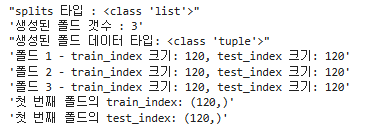
6) 학습 및 테스트 시퀀스 데이터 준비와 스케일링
def prepare_scaled_sequences(df, features, target_col, seq_length, train_index, test_index):

    df_train = df.iloc[train_index]
    train_data_X = df_train[features]
    train_data_Y = df_train[target_col]

    scaler_x = StandardScaler()
    scaler_y = StandardScaler()

    train_data_X_scaled = scaler_x.fit_transform(train_data_X)
    train_data_Y_scaled = scaler_y.fit_transform(train_data_Y)

    df_train_scaled = pd.DataFrame(train_data_X_scaled, columns=features, index=train_data_X.index)
    df_train_scaled[target_col] = train_data_Y_scaled

    df_test = df.iloc[test_index]
    test_data_X = df_test[features]
    test_data_Y = df_test[target_col]

    test_data_X_scaled = scaler_x.transform(test_data_X)
    test_data_Y_scaled = scaler_y.transform(test_data_Y)

    df_test_scaled = pd.DataFrame(test_data_X_scaled, columns=features, index=test_data_X.index)
    df_test_scaled[target_col] = test_data_Y_scaled

    sequence_dataX_train, sequence_dataY_train = build_sequence_dataset(df_train_scaled, target_col, seq_length)
    sequence_dataX_test, sequence_dataY_test = build_sequence_dataset(df_test_scaled,  target_col, seq_length)

    return sequence_dataX_train, sequence_dataY_train, sequence_dataX_test, sequence_dataY_test, (scaler_x, scaler_y)
7) 데이터 로더 생성 및 확인
from torch.utils.data import TensorDataset, DataLoader
def create_data_loaders_from_sequences(sequence_dataX_train, sequence_dataY_train,
                                       sequence_dataX_test, sequence_dataY_test,
                                       batch_size):

    # 텐서로 데이터 변환
    train_X_tensor = torch.tensor(sequence_dataX_train, dtype=torch.float32)
    train_Y_tensor = torch.tensor(sequence_dataY_train.reshape(-1, 1), dtype=torch.float32)
    test_X_tensor = torch.tensor(sequence_dataX_test, dtype=torch.float32)
    test_Y_tensor = torch.tensor(sequence_dataY_test.reshape(-1, 1), dtype=torch.float32)

    # TensorDataset 생성
    train_dataset = TensorDataset(train_X_tensor, train_Y_tensor)
    test_dataset = TensorDataset(test_X_tensor, test_Y_tensor)

    # DataLoader 설정
    train_loader = DataLoader(train_dataset, batch_size=batch_size, shuffle=True)
    test_loader = DataLoader(test_dataset, batch_size=batch_size, shuffle=False)

    return train_loader, test_loader
8) Sliding Window를 이용한 Stacked LSTM 모델 학습 및 검증
# device 및 데이터설정
device = torch.device("cuda" if torch.cuda.is_available() else "cpu")
df_weather = df_weather_org[features].copy()


# 파라미터 설정
seed_value = 42
set_seed(seed_value)  # 위에서 정의한 함수 호출로 모든 시드 설정

num_output = 1
num_hidden = 10
num_features = len(features)

seq_length = 6  # 과거 6일의 데이터를 기반으로 다음날의 기온을 예측
batch_size = 32
dropout_rate = 0.2
learning_rate = 0.002

# Sliding Window 설정
train_size = 360
test_size = 120- sliding_window_split 함수를 이용하여 지정한 학습/테스트 데이터 크기 및 시퀀스 길이를 지정하여 교차 검증 폴드를 만듭니다.
- prepare_scaled_sequences 함수를 이용하여, 각 폴드별 학습 및 테스트 세트로 분할하고, 각 세트를 스케일링한 후 시퀀스 데이터로 변환합니다.
- create_data_loaders_from_sequences 함수를 이용하여, 각 폴드별 시퀀스 데이터를 텐서로 변환하고, 이를 DataLoader로 생성합니다.
- 각 폴드마다 Stacked LSTM 모델 인스턴스를 생성합니다.
- train 함수를 이용하여 모델을 학습시키고, validate_model 함수를 사용하여 검증 데이터셋에서 성능을 평가합니다.
- 학습 및 검증 손실을 추적하여 최적의 모델을 선택합니다.
- 실제값과 best 손실 epoch에서의 예측값을 원래 스케일로 복원합니다.
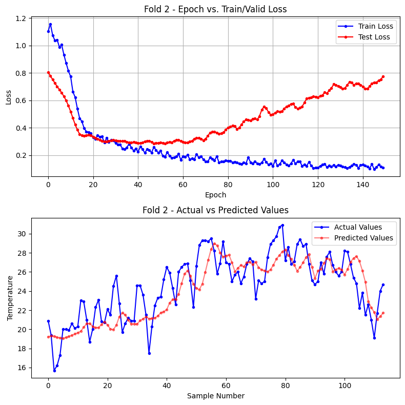
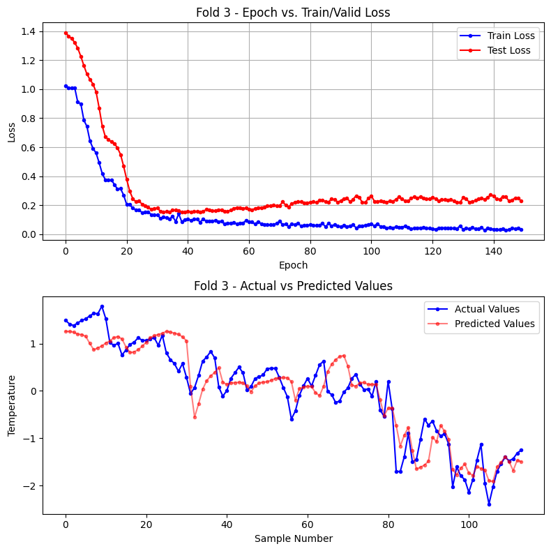
- plot_results 함수를 사용하여 각 폴드별 학습 및 검증 손실, 실제값과 예측값을 시각화합니다.
splits = sliding_window_split(df_weather.values, train_size, test_size, seq_length)

# 폴드별 성능 저장
fold_test_losses,fold_best_actuals_lst,fold_best_predictions_lst,fold_best_loss_lst,fold_best_epoch_lst = [],[],[],[],[]


for fold, (train_index, test_index) in enumerate(splits, start=1):
    print(f"Fold {fold}")
    print(f"Test data index: {test_index[0]} ~ {test_index[-1]} ")

    # 데이터 준비
    sequence_dataX_train, sequence_dataY_train, sequence_dataX_test, sequence_dataY_test, (scaler_x, scaler_y) = prepare_scaled_sequences(df_weather, features, target_col, seq_length, train_index, test_index)

    # DataLoader 생성
    train_loader, test_loader = create_data_loaders_from_sequences(
        sequence_dataX_train, sequence_dataY_train,
        sequence_dataX_test, sequence_dataY_test,
        batch_size = batch_size
    )
    # 모델 인스턴스 생성
    model_stackedLSTM = StackedLSTM(input_size=num_features, hidden_size=num_hidden, num_layers=2, output_size=num_output, dropout_rate = 0.2).to(device)

    optimizer_stackedLSTM = torch.optim.Adam(model_stackedLSTM.parameters(), lr=learning_rate)
    criterion_stackedLSTM = nn.MSELoss()

    # 학습
    train_loss_lst,test_loss_lst = [], []
    best_actuals, best_predictions = [], []  # 초기화

    best_loss = float('inf')
    max_epochs = 150

    for epoch in range(max_epochs):
        train_loss = train(model_stackedLSTM, train_loader, optimizer_stackedLSTM, criterion_stackedLSTM)
        test_loss, actuals, predictions = validate_model(model_stackedLSTM, test_loader, criterion_stackedLSTM)

        train_loss_lst.append(train_loss)
        test_loss_lst.append(test_loss)

        if test_loss < best_loss:
            best_loss = test_loss
            best_epoch = epoch
            best_actuals = actuals
            best_predictions = predictions

        if (epoch+1) % 10 == 0:
            print(f"epoch {epoch+1}: train loss(mse) = {train_loss:.4f}  test loss(mse) = {test_loss:.4f}")

    print(f"Fold {fold} 학습 완료 : 총 {epoch+1} epoch")

    actuals_original = scaler_y.inverse_transform(np.array(best_actuals).reshape(-1,1))
    best_predictions_original = scaler_y.inverse_transform(np.array(best_predictions).reshape(-1,1))

    fold_test_losses.append(test_loss)
    fold_best_actuals_lst.append(actuals_original)
    fold_best_predictions_lst.append(best_predictions_original)
    fold_best_loss_lst.append(best_loss)
    fold_best_epoch_lst.append(best_epoch)

    plot_results(train_loss_lst, test_loss_lst, actuals_original, best_predictions_original, fold)
Fold 1
Test data index: 370 ~ 489
epoch 10: train loss(mse) = 0.9546 test loss(mse) = 1.4176
epoch 20: train loss(mse) = 0.7920 test loss(mse) = 0.9752
epoch 30: train loss(mse) = 0.6838 test loss(mse) = 0.8483
epoch 40: train loss(mse) = 0.5995 test loss(mse) = 0.7651
epoch 50: train loss(mse) = 0.3875 test loss(mse) = 0.4702
epoch 60: train loss(mse) = 0.2914 test loss(mse) = 0.3813
epoch 70: train loss(mse) = 0.2591 test loss(mse) = 0.3055
epoch 80: train loss(mse) = 0.2134 test loss(mse) = 0.2626
epoch 90: train loss(mse) = 0.1885 test loss(mse) = 0.2700
epoch 100: train loss(mse) = 0.1925 test loss(mse) = 0.2890
epoch 110: train loss(mse) = 0.1570 test loss(mse) = 0.2786
epoch 120: train loss(mse) = 0.2029 test loss(mse) = 0.2914
epoch 130: train loss(mse) = 0.1449 test loss(mse) = 0.3210
epoch 140: train loss(mse) = 0.1229 test loss(mse) = 0.3643
epoch 150: train loss(mse) = 0.1330 test loss(mse) = 0.3627
Fold 1 학습 완료 : 총 150 epoch
Fold 2
Test data index: 490 ~ 609
epoch 10: train loss(mse) = 0.8152  test loss(mse) = 0.5614
epoch 20: train loss(mse) = 0.3600  test loss(mse) = 0.3446
epoch 30: train loss(mse) = 0.3091  test loss(mse) = 0.3099
epoch 40: train loss(mse) = 0.2473  test loss(mse) = 0.2913
epoch 50: train loss(mse) = 0.2176  test loss(mse) = 0.2888
epoch 60: train loss(mse) = 0.1668  test loss(mse) = 0.3030
epoch 70: train loss(mse) = 0.1695  test loss(mse) = 0.3091
epoch 80: train loss(mse) = 0.1627  test loss(mse) = 0.3852
epoch 90: train loss(mse) = 0.1850  test loss(mse) = 0.4570
epoch 100: train loss(mse) = 0.1403  test loss(mse) = 0.4959
epoch 110: train loss(mse) = 0.1664  test loss(mse) = 0.5751
epoch 120: train loss(mse) = 0.1087  test loss(mse) = 0.6241
epoch 130: train loss(mse) = 0.1297  test loss(mse) = 0.7039
epoch 140: train loss(mse) = 0.1296  test loss(mse) = 0.7131
epoch 150: train loss(mse) = 0.1108  test loss(mse) = 0.7760
Fold 2 학습 완료 : 총 150 epoch
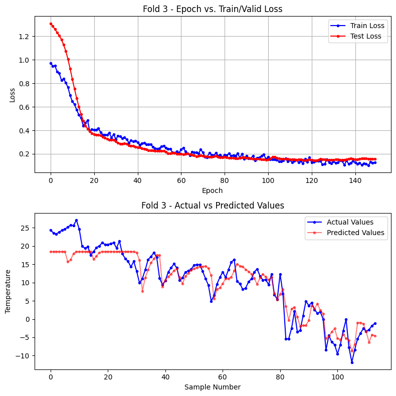
Fold 3
Test data index: 610 ~ 729
epoch 10: train loss(mse) = 0.6962  test loss(mse) = 0.9236
epoch 20: train loss(mse) = 0.4070  test loss(mse) = 0.3738
epoch 30: train loss(mse) = 0.3660  test loss(mse) = 0.3197
epoch 40: train loss(mse) = 0.3110  test loss(mse) = 0.2613
epoch 50: train loss(mse) = 0.2421  test loss(mse) = 0.2248
epoch 60: train loss(mse) = 0.2062  test loss(mse) = 0.1996
epoch 70: train loss(mse) = 0.2370  test loss(mse) = 0.1868
epoch 80: train loss(mse) = 0.1736  test loss(mse) = 0.1710
epoch 90: train loss(mse) = 0.1555  test loss(mse) = 0.1713
epoch 100: train loss(mse) = 0.1557  test loss(mse) = 0.1506
epoch 110: train loss(mse) = 0.1345  test loss(mse) = 0.1577
epoch 120: train loss(mse) = 0.1704  test loss(mse) = 0.1533
epoch 130: train loss(mse) = 0.1191  test loss(mse) = 0.1495
epoch 140: train loss(mse) = 0.1381  test loss(mse) = 0.1563
epoch 150: train loss(mse) = 0.1284  test loss(mse) = 0.1580
Fold 3 학습 완료 : 총 150 epoch
2. 양방향(Bidirectional) LSTM
1) 개요
기존의 시퀀스 데이터 학습 모델, 특히 LSTM(Long Short-Term Memory)과 GRU(Gated Recurrent Unit)는 주어진 시퀀스의 앞 부분(과거 정보)만을 사용하여 다음 값을 예측하는 데 중점을 두었습니다. 이는 시계열 데이터나 언어 모델에서 유용하지만, 시퀀스의 뒤쪽 부분(미래 정보)도 중요한 경우에는 한계를 가집니다.
전통적인 LSTM은 데이터를 한 방향으로만 처리합니다. 그러나 많은 실제 응용 분야에서는 데이터를 양방향으로 처리하는 것이 더 효과적일 수 있습니다. 예를 들어, 자연어 처리(NLP)에서는 문장의 앞뒤 문맥을 모두 이해하는 것이 중요하며, 음성 인식에서는 발음의 앞뒤 맥락을 모두 고려하는 것이 필요합니다. 이러한 요구를 해결하기 위해 양방향 순환 신경망(Bidirectional Recurrent Neural Network, BRNN)이 제안되었습니다.
1997년, Schuster와 Paliwal은 "Bidirectional Recurrent Neural Networks"라는 논문에서 양방향 RNN의 개념을 처음으로 제안했습니다. 이 모델은 입력 시퀀스를 양방향으로 처리하여 더 풍부한 정보를 학습할 수 있도록 설계되었습니다. BRNN은 두 개의 별도 RNN 레이어를 사용하여 입력 시퀀스를 정방향과 역방향으로 모두 학습하며, 두 방향의 출력을 결합하여 최종 출력을 생성합니다. 이를 통해 모델은 과거와 미래 정보를 모두 활용할 수 있습니다.
※ Bidirectional LSTM의 구조
Bidirectional LSTM의 구조는 다음과 같습니다. 입력 데이터는 두 개의 LSTM 층으로 전달되는데, 하나는 데이터를 정방향(순방향)으로 처리하고, 다른 하나는 역방향(반대 방향)으로 처리합니다. 이에 정방향 LSTM은 시퀀스를 처음부터 끝까지 처리하고, 역방향 LSTM은 시퀀스를 끝에서부터 처음까지 처리합니다.
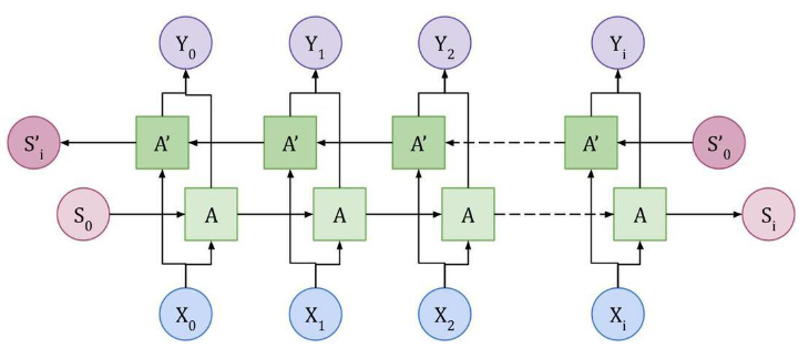
각 방향의 LSTM 층은 별도의 hidden state를 생성합니다. 즉, 정방향 LSTM은 정방향 hidden state를, 역방향 LSTM은 역방향 hidden state를 생성합니다. 이 두 방향의 hidden state는 최종적으로 결합되어(combine) 최종 출력을 만듭니다. 보통 이 결합 방식은 연결(concatenation)을 사용합니다.
예를 들어, 각 시점에서 정방향 LSTM의 hidden state가 ℎ→t이고, 역방향 LSTM의 hidden state가 ℎ←t이라면, 최종 출력은 (ℎ→t, ℎ←t)의 형태로 두 hidden state를 연결한 형태가 됩니다. 이 연결된 hidden state는 다음 층으로 전달되며 최적 예측 수행합니다.
이러한 구조는 단방향 LSTM보다 더 풍부한 표현력을 제공합니다. 왜냐하면, 양방향 LSTM은 시퀀스의 모든 시점에서 앞뒤 문맥 정보를 모두 고려하여 더 정확한 패턴을 학습할 수 있기 때문입니다.
2) nn.LSTM을 이용한 양방향(Bidirectional) LSTM 인스턴스 생성
import torch
import torch.nn as nn

# Bidirectional LSTM 인스턴스 생성 (드롭아웃 포함)
bilstm_ex1 = nn.LSTM(input_size=5, hidden_size=20, num_layers=2, bidirectional=True, dropout=0.5)

print(f"Input size : {bilstm_ex1.input_size}")
print(f"Hidden size : {bilstm_ex1.hidden_size}")
print(f"Number of layers : {bilstm_ex1.num_layers}")
print(f"Bidirectional : {bilstm_ex1.bidirectional}")
print(f"Dropout : {bilstm_ex1.dropout}")
Input size : 5
Hidden size : 20
Number of layers : 2
Bidirectional : True
Dropout : 0.5
3) Bidirectional LSTM을 이용한 시계열 예측 모델 만들기
import torch.nn as nn

class BiLSTMModel(nn.Module):
    def __init__(self, input_size, hidden_size, output_size, dropout_rate):
        super(BiLSTMModel, self).__init__()

        self.hidden_size = hidden_size
        self.bidirectional = True

        # 3개의 양방향 LSTM 레이어
        self.lstm1 = nn.LSTM(input_size, hidden_size, batch_first=True, bidirectional=self.bidirectional)
        self.dropout1 = nn.Dropout(dropout_rate)
        self.lstm2 = nn.LSTM(hidden_size * 2, hidden_size, batch_first=True, bidirectional=self.bidirectional)
        self.dropout2 = nn.Dropout(dropout_rate)
        self.lstm3 = nn.LSTM(hidden_size * 2, hidden_size, batch_first=True, bidirectional=self.bidirectional)
        self.dropout3 = nn.Dropout(dropout_rate)

        # 최종 출력을 위한 두 단계의 선형 레이어와 ReLU 활성화 함수
        self.fc1 = nn.Linear(hidden_size * 2, hidden_size // 2)
        self.relu = nn.ReLU()
        self.fc2 = nn.Linear(hidden_size // 2, output_size)

    def forward(self, x):
        # 데이터를 LSTM 레이어와 드롭아웃 레이어를 통과시킵니다
        x, _ = self.lstm1(x)
        x = self.dropout1(x)
        x, _ = self.lstm2(x)
        x = self.dropout2(x)
        x, _ = self.lstm3(x)
        x = self.dropout3(x)

        # 마지막 타임 스텝의 출력을 선형 레이어와 ReLU 활성화 함수로 전달
        x = self.fc1(x[:, -1, :])
        x = self.relu(x)
        x = self.fc2(x)
        return x

# 'bilstm_ex2' 변수명은 정답체크를 위해 수정하지 마세요
bilstm_ex2 = BiLSTMModel(input_size=5, hidden_size=20, output_size=1, dropout_rate=0.2)
bilstm_ex2
BiLSTMModel(
(lstm1): LSTM(5, 20, batch_first=True, bidirectional=True)
(dropout1): Dropout(p=0.2, inplace=False)
(lstm2): LSTM(40, 20, batch_first=True, bidirectional=True)
(dropout2): Dropout(p=0.2, inplace=False)
(lstm3): LSTM(40, 20, batch_first=True, bidirectional=True)
(dropout3): Dropout(p=0.2, inplace=False)
(fc1): Linear(in_features=40, out_features=10, bias=True)
(relu): ReLU()
(fc2): Linear(in_features=10, out_features=1, bias=True)
)
4) 양방향(Bidirectional LSTM) 모델 학습과 교차 검증, 시각화
# device 및 데이터설정
device = torch.device("cuda" if torch.cuda.is_available() else "cpu")
df_weather = df_weather_org[features].copy()
# 파라미터 설정
seed_value = 42
set_seed(seed_value) # 위에서 정의한 함수 호출로 모든 시드 설정
num_output = 1
num_hidden = 10
num_features = len(features)
seq_length = 6 # 과거 6일의 데이터를 기반으로 다음날의 기온을 예측
batch_size = 32
dropout_rate = 0.2
learning_rate = 0.005
# Sliding Window 설정
train_size = 360
test_size = 120
# 폴드별 성능 저장
fold_test_losses,fold_best_actuals_lst,fold_best_predictions_lst,fold_best_loss_lst,fold_best_epoch_lst = [],[],[],[],[]
for fold, (train_index, test_index) in enumerate(splits, start=1):
print(f"Fold {fold}")
print(f"Test data index: {test_index[0]} ~ {test_index[-1]} ")
# 데이터 준비
sequence_dataX_train, sequence_dataY_train, sequence_dataX_test, sequence_dataY_test, (scaler_x, scaler_y) = prepare_scaled_sequences(df_weather, features, target_col, seq_length, train_index, test_index)
# DataLoader 생성
train_loader, test_loader = create_data_loaders_from_sequences(
sequence_dataX_train, sequence_dataY_train,
sequence_dataX_test, sequence_dataY_test,
batch_size = 32
)
# 모델 인스턴스 생성
model_BiLSTM = BiLSTMModel(input_size=num_features, hidden_size=num_hidden, output_size=num_output, dropout_rate = 0.2).to(device)
optimizer_BiLSTM = torch.optim.Adam(model_BiLSTM.parameters(), lr=learning_rate)
criterion_BiLSTM = nn.MSELoss()
# 학습
train_loss_lst,test_loss_lst = [], []
best_actuals, best_predictions = [], [] # 초기화
best_loss = float('inf')
max_epochs = 150
for epoch in range(max_epochs):
train_loss = train(model_BiLSTM, train_loader, optimizer_BiLSTM, criterion_BiLSTM)
test_loss, actuals, predictions = validate_model(model_BiLSTM, test_loader, criterion_BiLSTM)
train_loss_lst.append(train_loss)
test_loss_lst.append(test_loss)
if test_loss < best_loss:
best_loss = test_loss
best_epoch = epoch
best_actuals = actuals
best_predictions = predictions
if (epoch+1) % 10 == 0:
print(f"epoch {epoch+1}: train loss(mse) = {train_loss:.4f} test loss(mse) = {test_loss:.4f}")
print(f"Fold {fold} 학습 완료 : 총 {epoch+1} epoch")
actuals_original = scaler_y.inverse_transform(np.array(best_actuals).reshape(-1,1))
best_predictions_original = scaler_y.inverse_transform(np.array(best_predictions).reshape(-1,1))
fold_best_actuals_lst.append(actuals_original)
fold_best_predictions_lst.append(best_predictions_original)
fold_best_loss_lst.append(best_loss)
fold_best_epoch_lst.append(best_epoch)
plot_results(train_loss_lst, test_loss_lst, best_actuals, best_predictions, fold)
print("-----------------------------------------------------")
for fold in range(len(splits)):
print(f"폴드 {fold} best 테스트 손실 (MSE) : {round(np.mean(fold_best_loss_lst[fold]),4)} at {best_epoch} epoch: ")
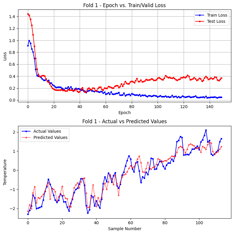
print(f"폴드 테스트 평균 손실 (MSE) : {round(np.mean(fold_best_loss_lst),4)}")Fold 1
Test data index: 370 ~ 489
epoch 10: train loss(mse) = 0.3991 test loss(mse) = 0.3947
epoch 20: train loss(mse) = 0.2554 test loss(mse) = 0.1977
epoch 30: train loss(mse) = 0.2024 test loss(mse) = 0.1528
epoch 40: train loss(mse) = 0.1908 test loss(mse) = 0.1333
epoch 50: train loss(mse) = 0.1589 test loss(mse) = 0.1719
epoch 60: train loss(mse) = 0.1317 test loss(mse) = 0.2015
epoch 70: train loss(mse) = 0.1132 test loss(mse) = 0.2431
epoch 80: train loss(mse) = 0.0804 test loss(mse) = 0.3051
epoch 90: train loss(mse) = 0.0805 test loss(mse) = 0.3109
epoch 100: train loss(mse) = 0.0694 test loss(mse) = 0.3407
epoch 110: train loss(mse) = 0.0493 test loss(mse) = 0.3799
epoch 120: train loss(mse) = 0.0675 test loss(mse) = 0.3742
epoch 130: train loss(mse) = 0.0670 test loss(mse) = 0.3544
epoch 140: train loss(mse) = 0.0440 test loss(mse) = 0.3465
epoch 150: train loss(mse) = 0.0511 test loss(mse) = 0.3736
Fold 1 학습 완료 : 총 150 epoch
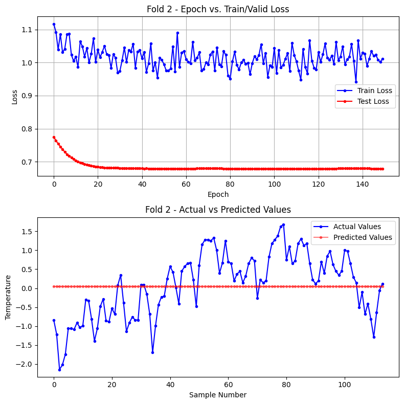
Fold 2
Test data index: 490 ~ 609
epoch 10: train loss(mse) = 1.0049  test loss(mse) = 0.7085
epoch 20: train loss(mse) = 1.0015  test loss(mse) = 0.6856
epoch 30: train loss(mse) = 0.9691  test loss(mse) = 0.6816
epoch 40: train loss(mse) = 1.0370  test loss(mse) = 0.6803
epoch 50: train loss(mse) = 1.0081  test loss(mse) = 0.6796
epoch 60: train loss(mse) = 1.0345  test loss(mse) = 0.6797
epoch 70: train loss(mse) = 0.9999  test loss(mse) = 0.6802
epoch 80: train loss(mse) = 0.9602  test loss(mse) = 0.6796
epoch 90: train loss(mse) = 0.9646  test loss(mse) = 0.6791
epoch 100: train loss(mse) = 0.9863  test loss(mse) = 0.6796
epoch 110: train loss(mse) = 1.0226  test loss(mse) = 0.6793
epoch 120: train loss(mse) = 0.9789  test loss(mse) = 0.6790
epoch 130: train loss(mse) = 1.0072  test loss(mse) = 0.6799
epoch 140: train loss(mse) = 1.0115  test loss(mse) = 0.6803
epoch 150: train loss(mse) = 1.0118  test loss(mse) = 0.6796
Fold 2 학습 완료 : 총 150 epoch
Fold 3
Test data index: 610 ~ 729
epoch 10: train loss(mse) = 0.5913  test loss(mse) = 1.0347
epoch 20: train loss(mse) = 0.2699  test loss(mse) = 0.4687
epoch 30: train loss(mse) = 0.1326  test loss(mse) = 0.1756
epoch 40: train loss(mse) = 0.1007  test loss(mse) = 0.1551
epoch 50: train loss(mse) = 0.0942  test loss(mse) = 0.1610
epoch 60: train loss(mse) = 0.0941  test loss(mse) = 0.1808
epoch 70: train loss(mse) = 0.0767  test loss(mse) = 0.1952
epoch 80: train loss(mse) = 0.0616  test loss(mse) = 0.2166
epoch 90: train loss(mse) = 0.0567  test loss(mse) = 0.2215
epoch 100: train loss(mse) = 0.0664  test loss(mse) = 0.2481
epoch 110: train loss(mse) = 0.0480  test loss(mse) = 0.2569
epoch 120: train loss(mse) = 0.0405  test loss(mse) = 0.2459
epoch 130: train loss(mse) = 0.0597  test loss(mse) = 0.2199
epoch 140: train loss(mse) = 0.0372  test loss(mse) = 0.2741
epoch 150: train loss(mse) = 0.0336  test loss(mse) = 0.2308
Fold 3 학습 완료 : 총 150 epoch
-----------------------------------------------------
폴드 0 best 테스트 손실 (MSE) : 0.1333  at 38 epoch:
폴드 1 best 테스트 손실 (MSE) : 0.679  at 38 epoch:
폴드 2 best 테스트 손실 (MSE) : 0.1517  at 38 epoch:
폴드 테스트 평균 손실 (MSE) : 0.3213'딥러닝 > 딥러닝: 시계열 데이터' 카테고리의 다른 글
| 시계열 교차검증 (TimeSeries Split & Sliding Window Split) (0) | 2025.01.29 |
|---|---|
| LSTM 종합 코드 정리 (0) | 2025.01.28 |
| LSTM 학습과 추론, 모델 저장과 복원 (0) | 2025.01.24 |
| LSTM 모델 생성과 연속적 sequence 데이터 처리 (0) | 2025.01.23 |
| LSTM 원리와 구조 및 LSTMcell 구현 (0) | 2025.01.23 |